Chapter 3 delves extensively into the loads and generation of electrical power. It addresses the long-term, medium-term, and short-term behavior of the load. Specifically, the stochastic behavior of the load in the short term is explained. Additionally, new developments in consumption and decentralized generation are discussed.
The translation of ‘Networks for Electricity Distribution’ was created with the help of artificial intelligence and carefully reviewed by subject-matter experts. Even with our combined efforts, a few inaccuracies may still remain. If you notice anything that could be improved, we’d love to hear from you.
Knowledge of loads and generation is a fundamental requirement for power system planning and designing a distribution network. For designing a distribution network that must be economically viable years into the future, it is necessary to base the design on well-founded assumptions regarding the demanded and produced power and their development. The network planner must demonstrate through calculations that the design will result in a technical and economic optimum. In these calculations, the planner must be able to handle, on one hand, large quantities of similarly behaving loads and small decentralized generation units, and on the other hand, small quantities of dissimilarly behaving large loads and generation units.
A distribution network is designed to provide uninterrupted electrical power of sufficient quality to its users for more than 40 years into the future. The energy transition will lead to the connection of new loads and generators, such as large numbers of heat pumps, µCHPs (Combined Heat and Power), solar panels, a gradually increasing number of electric cars, and battery- and air conditioning-systems. The future distribution network must be designed in such a way that major adjustments can be avoided. Therefore, knowledge of the development of load and generation is of great importance.
The load is categorized into various types. This categorization includes an analysis of behavior as a function of time and as a function of the network voltage. The voltage-dependent behavior is discussed in the chapter on modeling. This chapter primarily addresses behavior over time, for short, medium, and long terms. The short term refers to the instantaneous behavior within a maximum of about one hour. The medium term refers to behavior over a limited period without growth, such as one day or one week. The long term refers to a period of several years, possibly in combination with periodic medium-term behavior.
There are many conceivable ways to categorize the loads. Each company uses its own method. A commonly used method is (EnergieNed, 1996):
1. small business consumption
2. household small consumption
a. detached houses
b. single-family homes
c. apartments
3. mixed small consumption (business and household)
It is inevitable that particularly in the category of ‘small business consumption,’ the diversity can be large. Loads in the category of ‘household small consumption’ will exhibit a much more uniform character. Nothing can be said in advance about the category of ‘mixed small consumption’, as it depends both on the type of business consumption and the distribution between business and household consumption. A more precise definition of these categories will have to be made by the network designer themselves. This, of course, depends on the level of accuracy one expects to achieve and the available data.
Loads in the categories of commercial or household consumption exhibit similar behavior throughout the year. Specific loads, such as heat pumps and electric cars, place high demands on the distribution network and require a special approach. Loads in the ‘heat pumps’ category will consume a lot of electricity, particularly during the cold period. Loads in the ‘electric cars’ category will consume a lot of electricity, especially after the morning and evening rush hours.
It should be noted here that decentralized generation deserves special attention. In locations where µCHP (Combined Heat and Power) or solar panels are widely used, decentralized generation plays a significant role in considerations regarding the power load on the distribution network. Depending on the concentrations, the power flow in the distribution network can be compensated or even change direction. A connection can both receive and supply power.
The loads in a distribution network exhibit annual growth. The growth is usually indicated as a percentage relative to the start date. Distribution networks are dimensioned in such a way that the accretion within the economic lifespan does not lead to major adjustments or with a well-defined expansion path. This means that the networks are designed for the maximum load that occurs at the end of their economic lifespan. For the forecast, the network planner must have insight into:
The number of connections is primarily determined by planning from the national to the regional level. For the higher network levels, such as transformers and medium-voltage networks, the increase is largely due to load growth resulting from the rise in the number of connections. There is a simple approach that uses the number of connections and the average annual consumption of the specific type of connection.
In addition to the increase in the number of connections, a forecast of the load and generation development of existing connections is important. This requires estimates and decisions regarding:
The future behavior of the customer is almost impossible to predict in detail. Therefore, it is usually sufficient to extrapolate historical data from categories of customers, possibly adjusted by professional and political insight. In doing so, the network planner relies on planning information and market analysis. There is no universally applicable model or forecasting system. The uncertainties are greatest in low-voltage networks. As a result, network designers tend to increasingly hedge against future uncertainties by designing the low-voltage network as robustly as possible: with maximum cable cross-sections and the largest possible distribution transformer, for example, 630 kVA. Additionally, in new constructions, the designer will claim extra space to potentially place additional network spaces in the future if necessary, thereby avoiding future grid expansion costs as much as possible.
The technical developments in equipment are primarily focused on increasing efficiency, which should lead to energy savings. Think of energy-efficient lighting, for example. On the other hand, new equipment is being developed that, while efficient in energy use, consumes much more electricity. The rise of new types of loads such as heat pumps and electric cars also has a significant impact on growth. The lower the network level, the greater this influence is. Decentralized generation is also a complicating factor for the forecast.
The possibilities for energy management systems are becoming relevant again due to developments in the field of ‘smart grids’. These developments mostly pertain to balancing the voltage and the supply and demand of electrical energy.
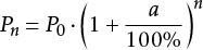
Figure 3.1 shows the development of electricity consumption in the Netherlands from 1938 to 2008 (source: CBS 2010). Noteworthy is the trend break around the year 1973. As a result, the growth over the entire period is roughly divided into two time frames. In the first period, from 1938 to 1973, the growth was 8% annually. From 1973 to 2008, the growth was 2.4% per year. This is based on exponential growth:
|
[ |
3.1 |
] |
The graph shows the figures recorded by CBS and the calculated curve with the growth rates mentioned above.
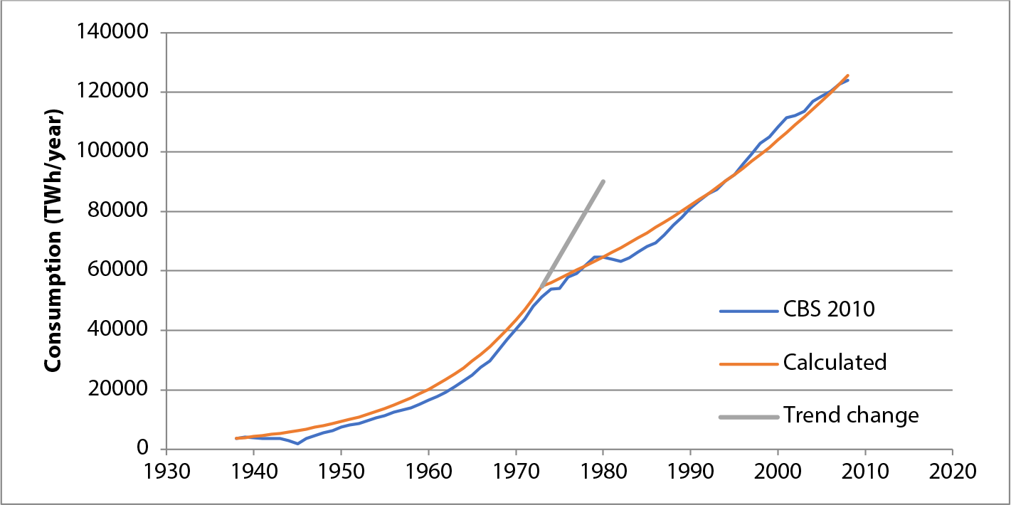
A period of 70 years is usually too long for a reasonable growth forecast. There is a clear trend break around 1973. Figure 3.2 shows the development of electricity consumption in the Netherlands from 1995 to 2008. A linear trend line has been added to the graph. Over this 13-year period, the increase relative to 1995 is approximately linear at 2.4% per year.
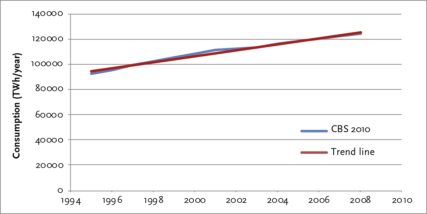
Figure 3.3 shows the consumption in the Netherlands in 2008. The difference between summer and winter is about 20 percent. This graph indicates that within the span of one year, growth is typically not taken into account. However, seasonal behavior is considered.
The medium term is a flexible concept. The load can be assumed to be known to some extent during this period, as growth and random behavior play a lesser role. The behavior of the load is then called deterministic. Medium term behavior describes the load over a day, a week, a month, or a portion of a year. Depending on the application, the network planner uses the maximum and minimum values of the load or uses load patterns.
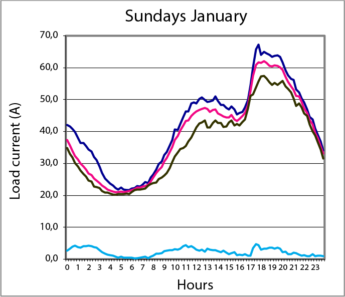
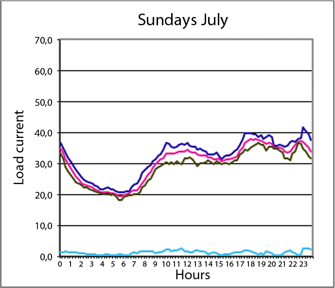
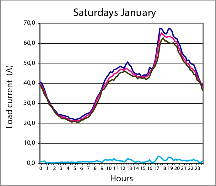
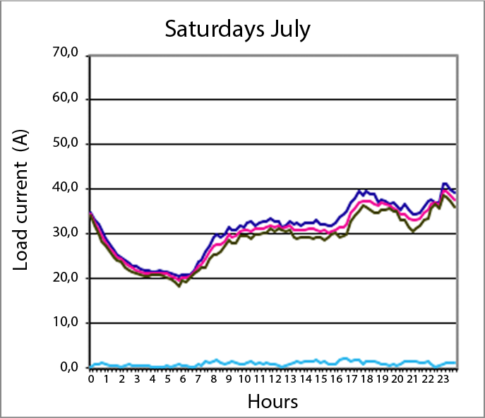
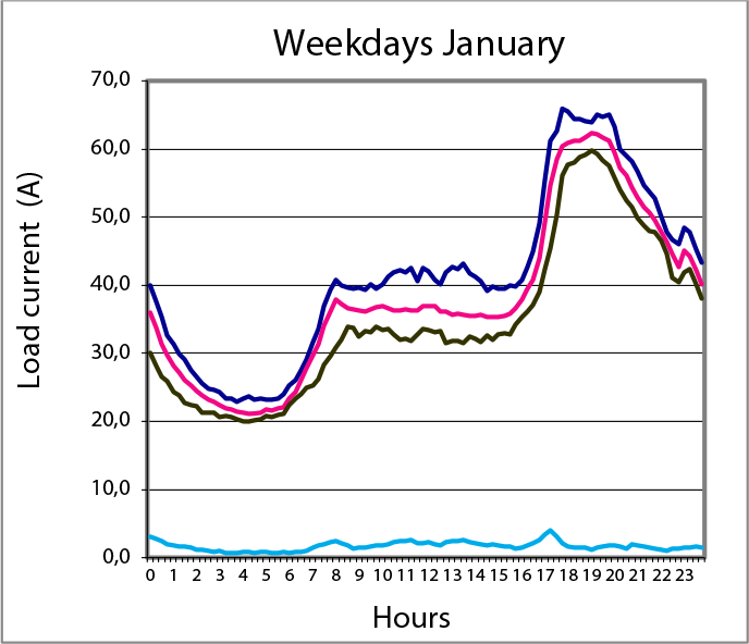
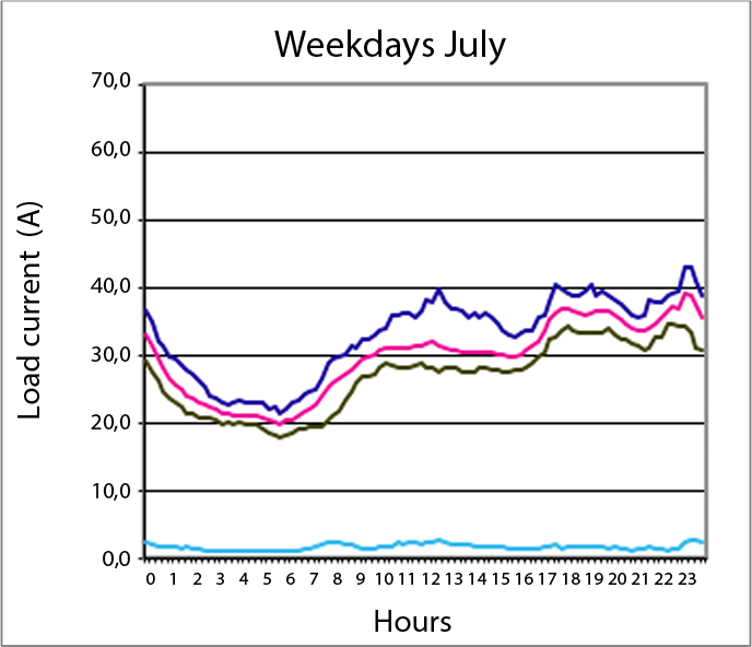
Figure 3.4 (above) provides an example of the power flows in a residential area during the winter (left) and the summer (right). This residential area only has ‘traditional’ loads. That is to say: regular household appliances and lighting, and no electric cars, heat pumps, µCHP units, or solar panels. The loads on Sunday, Saturday, and weekdays are very similar, both in winter and summer. For all days of the week, the maximum in the summer is approximately 60% of the winter maximum. The minimum in the summer is roughly equal to the winter minimum. In the shape of the daily load curve in the winter, the behavior in the evening hours is clearly visible. Generally, between 5:00 PM and 10:00 PM, the load is significantly higher than during the day.
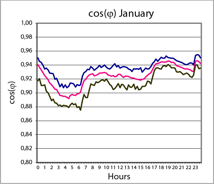
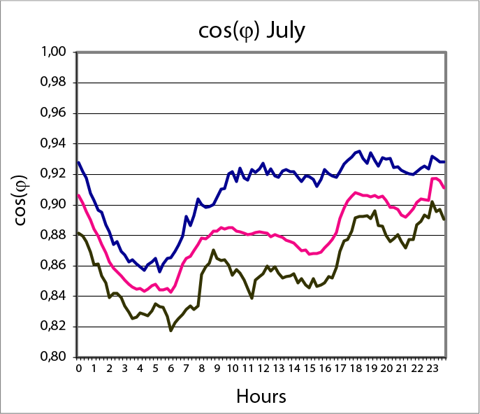
Figure 3.5 illustrates the behavior of the power factor cos(φ) over the weekdays in January (left) and July (right). It is noticeable that the power factor averages 0.92 in the winter and 0.88 in the summer. During periods of low load, the power factor shows lower values than during periods of high load.
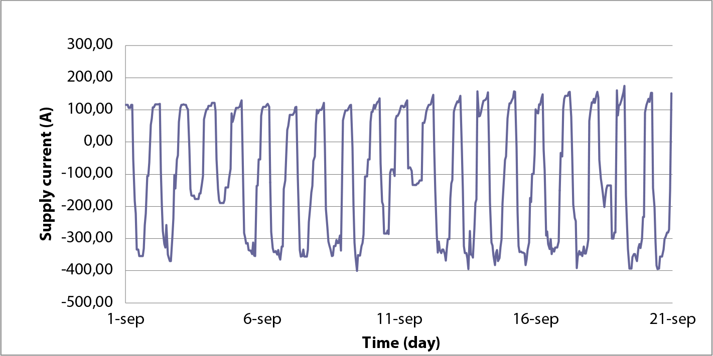
The load patterns can be applied to a short time span, such as a day, but also for a longer time span, such as a month or a year. Figure 3.6 shows the behavior of the supply current from the substation of a 20 kV line to a greenhouse area over three weeks in September. A negative value of the current means a reverse energy direction. It is clearly visible that the current changes sign daily. This means that the sum of the current of all connected users alternates daily between consumption and local production. In this case, a load current of 100 A corresponds to a three-phase power of approximately 3.5 MVA.
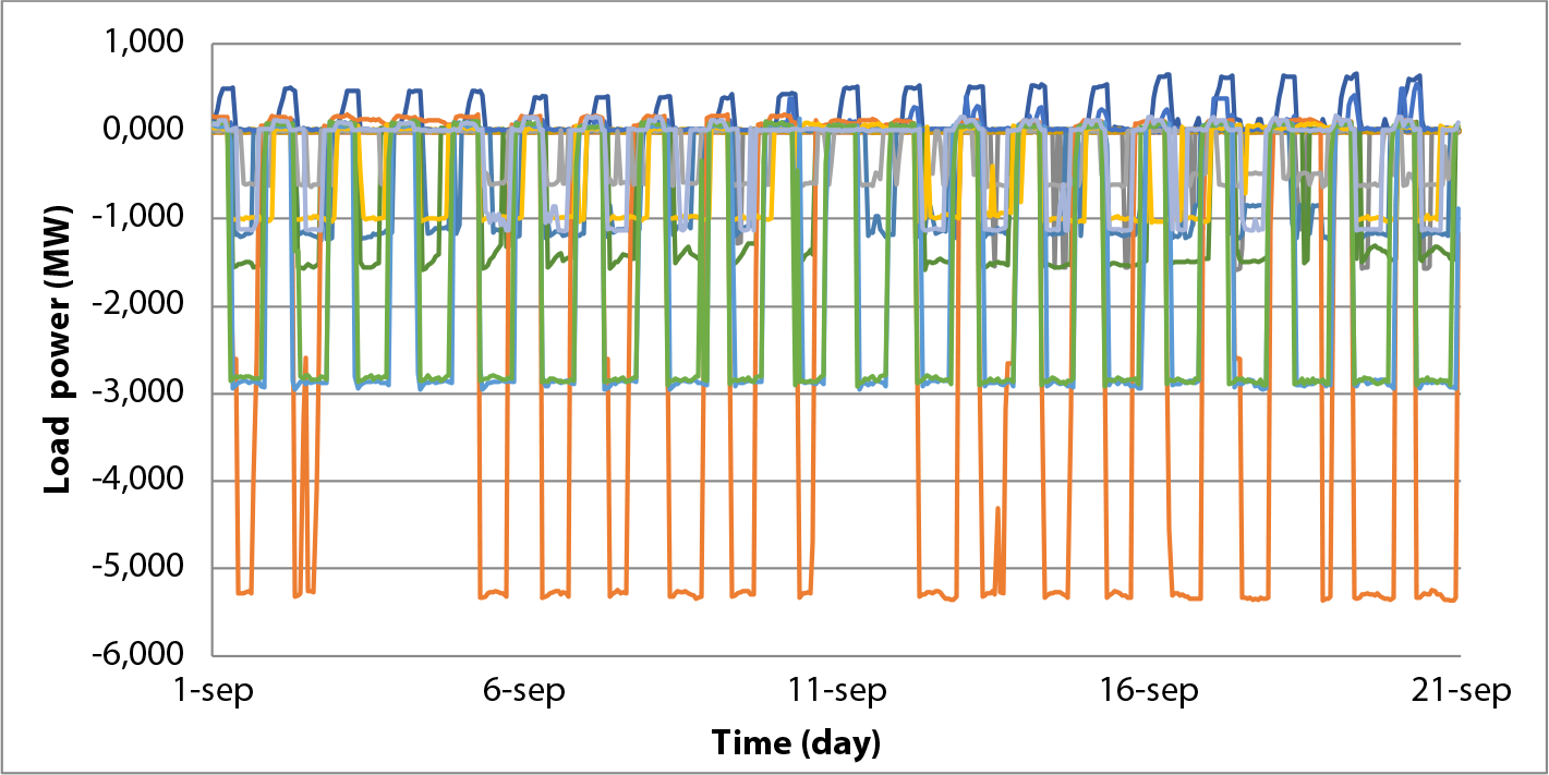
Measurement of the loads at the individual nodes shows how the total supply current of the feeder is composed of the sum of all loads and generators. The graphs of the generator capacities demonstrate how the switching on and off of decentralized generation leads to daily fluctuations of up to over 5 MW per generator.
The short-term behavior of the load aims to predict the load at the time of the minimum, maximum, or another specific moment. The load consists of a portion that is fairly predictable (the medium term) and a portion where the load behaves randomly. For a residential area, it is reasonably well known when the minimum and maximum load occurs and what the expected value of that load is. Additionally, there is always a certain random component that ensures the maxima of all individual loads never occur simultaneously, and thus the maximum of the sum of all loads is never equal to the sum of all maxima.
The following paragraphs will further explain the concepts of ‘stochastic behavior’ and ‘simultaneity’ of the load. In existing networks without electric cars, heat pumps, micro-CHPs, and solar panels, the described technique accounts for the non-simultaneity of the loads. However, in networks with electric cars, heat pumps, micro-CHPs, and solar panels, one cannot rely solely on the non-simultaneous behavior of the load. In addition to the stochastic behavior, a significant component of the load that behaves with high simultaneity must also be considered. For instance, if uncontrolled electric cars will be charged upon returning home at the end of a workday, and heat pumps with possible auxiliary heating will all operate simultaneously on cold days. As a result, the design of new networks will increasingly be based on the sum of the individual maximum loads, with only limited consideration given to stochastic behavior.
Individual customers exhibit a certain group behavior in electricity consumption over a 24-hour period, but at any given moment, they behave as independent individuals. After all, not everyone runs their washing machine at the same time. However, individual users, as a function of time spread over a day, generally show significant similarities in behavior. Figure 3.8, where the load curves are normalized to their average, illustrates this. Between 1:00 AM and 7:00 AM, the load is minimal. Between 7:00 AM and 9:00 AM, the load increases rapidly. In the evening, the load increases even more, only to decrease again to the minimum.
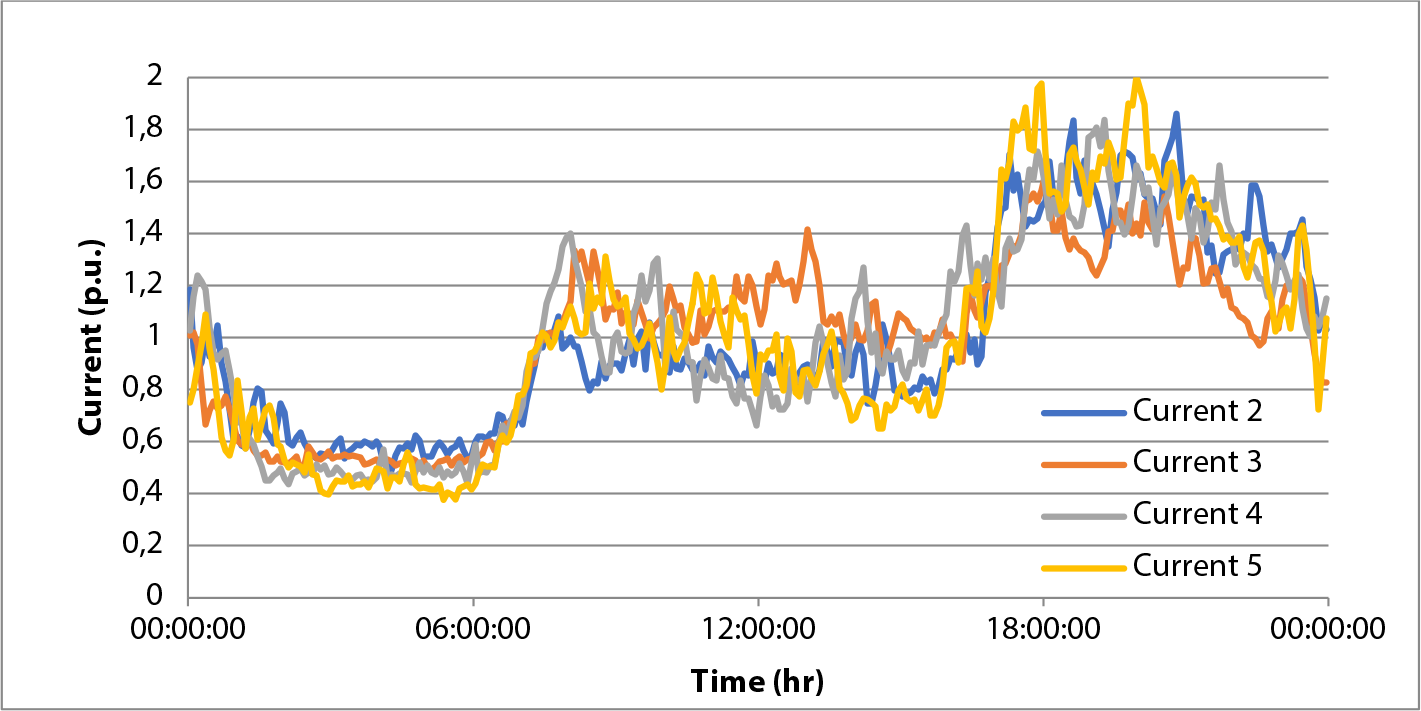
The behavior of the loads is described by the deterministic behavior as a function of time and the instantaneous stochastic parameters, which are independent. The deterministic behavior is described with a pattern as a function of time. An obvious pattern is a 24-hour daily load curve. The load curves for groups of loads are now reasonably well known through measurement projects.
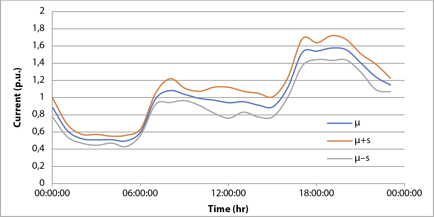
All loads behave as mutually dependent stochastic signals over the entire day, but within a limited time window (for example, one hour), they behave as independent stochastic signals. For these independent stochastic signals, an average value and a standard deviation (std, σ) can be calculated per time window. Figure 3.9 illustrates this. From all normalized load curves, load curves based on hourly averages were first calculated. These hourly curves were then plotted as a function of time. For each hourly value, the standard deviation between all four curves was calculated. This standard deviation was plotted as a function of time.
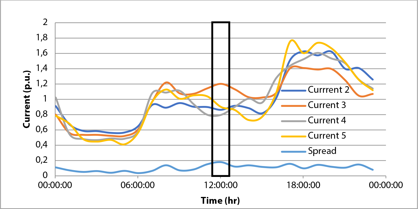
In figure 3.9, the t=12:oo h time window is indicated. Within that time window, the instantaneous load behaves as an independent stochastic signal. The load can be described in each time window as a stochastic variable, with an average value and a standard deviation. For the indicated time window in figure 3.9, the average value of the current is approximately equal to 1 p.u. and the standard deviation is approximately equal to 0.2 p.u.
The Central Limit Theorem states that the probability distribution of the sum of a sufficiently large number of independent stochastic variables is approximately normally distributed. This means, in this case, that the sum of a sufficient number of independent stochastic load signals behaves approximately like a normal distribution. This is confirmed by Engels (RWTH, 2000) and Livik (CIRED, 1993).
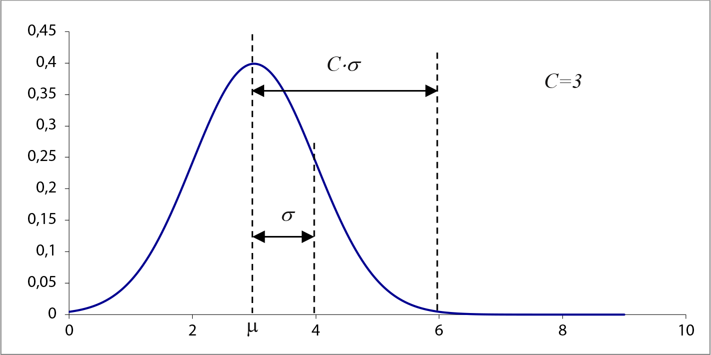
With this assumption, the load at a given timestamp ‘t’ can be described by a normal probability distribution with a mean μ(t) and standard deviation σ(t). Figure 3.10 shows the probability distribution for a load with an average value of 3 kW and a standard deviation of 1 kW.
The load model is completed by representing the mean values and the standard deviations as functions of time. This describes the behavior of the load for any desired period through a profile of stochastic normal distributions, characterized by the time functions for the means μ(t) and for the deviations σ(t) .
This modeling applies to similar types of loads. Other types of loads must be modeled separately, each with their own time functions. For mixed loads, combinations of the separate time functions must be used. Special loads, such as heavy industry, agricultural enterprises, and electric traction, as well as decentralized generators, continue to require special attention and cannot be modeled using this method.
Figure 3.11 shows the average load curve for the aforementioned four loads. This curve is labeled ‘μ’. Additionally, a band has been indicated, within which the individual load curves will likely fall with a certain probability. The upper and lower limits are calculated by adding the standard deviation to the average curve (labeled ‘μ+s’) and subtracting it (labeled ‘μ–s’), respectively. If the stochastic load behaves as a normally distributed stochastic variable at all times, the actual value of the load would fall within the indicated limits with a probability of approximately 70%.
All loads modeled in this strict manner can be summed according to the theory of stochastic signals. This has implications for the mean and the variance.
Figure 3.12 illustrates how this works out in a distribution network. Each graph shows the probability distribution of the power flow for the beginning, middle, and end of a feeder, respectively. The average values are 50, 20, and 5, respectively. The standard deviation increases towards the end of the feeder.
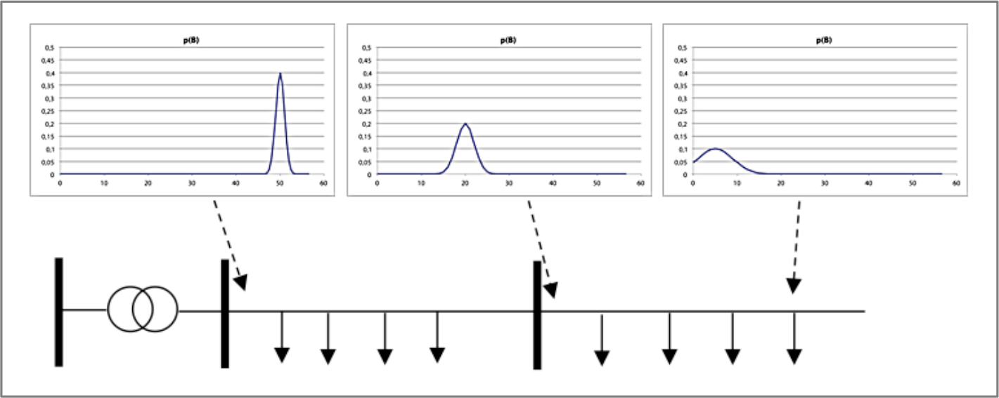
Close to the feeder, the number of loads, and thus the number of independent stochastic signals, is large. As the sum of the number of independent loads decreases further in the network, the uncertainty (and thus the standard deviation) increases. This is because the maximum load for different consumers will occur at different times. This phenomenon was previously described by Rusck. Therefore, we see that the average value decreases and the standard deviation proportionally increases. A study has shown that for outgoing directions in the low-voltage network, the number of connections is too small to apply the normal distribution. A notable result of this study was that around peak load moments, 20% of the connections were responsible for 50% of that peak (Provoost, 2011). For a small number of consumers, it is therefore no longer correct to apply the normal distribution.
For each specific moment of the day, the load size of a specific category can be approximately predicted. The deterministic part is described using patterns for, for example, a day. This way, the moments when the load is minimal or maximal can be estimated. These are important values for sizing a distribution network. However, a distribution network is not sized for the sum of the individual maximum load values of all connections because the maximum load of the individual connections will occur at different times. This phenomenon is called diversity or non-simultaneity.
Design calculations for low-voltage (LV) and medium-voltage (MV) networks are typically performed using maximum loads in combination with diversity factors. The technique is based on information that distribution companies gather annually through consumption and maximum load measurements at various points in the network.
The maximum load Pmax is defined as the highest value of the load for connections, cables, or transformers. An index indicates the number of connections to which the maximum load applies. The value is expressed in kW.
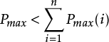
Diversity (or non-simultaneity) is the phenomenon where the maximum load at a point in the distribution network is smaller than the sum of the individual maximum loads of the connections or of the points fed from the considered point. Diversity occurs both for all connections that are connected to a feeder or a substation and for all feeders that are connected to a substation.
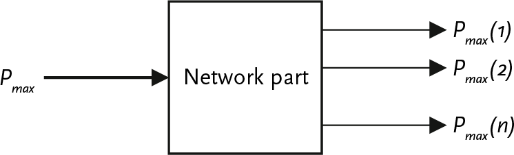
In figure 3.13, Pmax is the feeder current and Pmax(i) the maximum load in direction i. For this (radially operated) network, the following applies:
|
[ |
3.2 |
] |
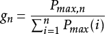
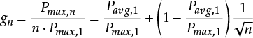
The relationship that calculates the maximum load of a part of the distribution network using the simultaneity factor was described by Rusck in 1956. The model assumes that the loads behave as statistically independent variables with a normal probability distribution. The purpose of the model is to determine the maximum load of components, such as cables or a supply transformer, using diversity. The degree of diversity is described by the simultaneity factor s, which is defined as the quotient of the maximum load Pmax,n for n connections and the sum of the maximum values Pmax(i) of the individual loads that are fed from this point.
|
[ |
3.3 |
] |
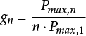
For n equal loads with maximum power Pmax,1 equation 3.3 becomes:
|
[ |
3.4 |
] |
in other words:
 |
[ |
3.5 |
] |
One of the conditions for applying Rusck’s model is that all loads behave as mutually independent normally distributed stochastic variables. However, when considered over an entire day, the load does not behave as a normally distributed stochastic variable. Generally, two time windows can be identified for peak and off-peak loads. Within one time window, it can be assumed that the load behaves as a normally distributed stochastic variable. This specific time window preferably occurs during peak load. According to probability theory, the stochastic variable can be described with the average value in the time window and a corresponding standard deviation. The difference between the maximum load and the average load in the time window is then proportional to the standard deviation. For a single connection, the following applies:
|
[ |
3.6 |
] |
in which:
| Pmax,1 | maximum load of a single user |
| Pavg,1 | average load of a single user |
| σ1 | standard deviation of a single user |
| C | a constant factor |
In a normal distribution, theoretically, the maximum of the argument of the normal distribution (the load value) is infinite. However, the maximum value of the load in the distribution network is indeed finite. The factor C defines the relationship between, on the one hand, the difference between the maximum and the average of the load and, on the other hand, the standard deviation from the probability concept. See figure 3.10, where C=3.
For a simultaneous load of n connections, the same factor applies C:
|
[ |
3.7 |
] |
Because the load for each similar connection behaves as the same normal distribution, the standard deviation applies to n connections:
|
[ |
3.8 |
] |
and for the average load of n connections:
|
[ |
3.9 |
] |
After combination, the following results from the above equations:

|
[ |
3.10 |
] |
By dividing equation 3.10 by n·Pmax,1 the expression for the simultaneity factor follows:
|
[ |
3.11 |
] |
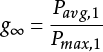
For an infinite number of connections, the following applies:
|
[ |
3.12 |
] |
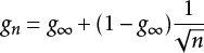
The simultaneity factor for an infinite number of connections describes the behavior for a specific load type, independent of the number of connections. Thus, the equation for the simultaneity factor transforms into the Rusck equation:
 |
[ |
3.13 |
] |
As a result, the formula for the maximum load can also be written as:

|
[ |
3.14 |
] |
For one connection, it is n=1 and is the simultaneity factor g1=1. For an infinite number of connections applies n→∞ and gn=g∞. In practice, it appears g∞ to be approximately equal for most cases to 0.2. In that case, the simultaneity factor gn is for 80% proportional to the inverse of the square root of the number of consumers.
The simultaneity factor strongly depends on the homogeneity of the load. For a highly homogeneous load, such as public lighting, the factor will be approximately equal to 1. The size of the considered network segment also has a significant impact on the value.
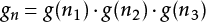
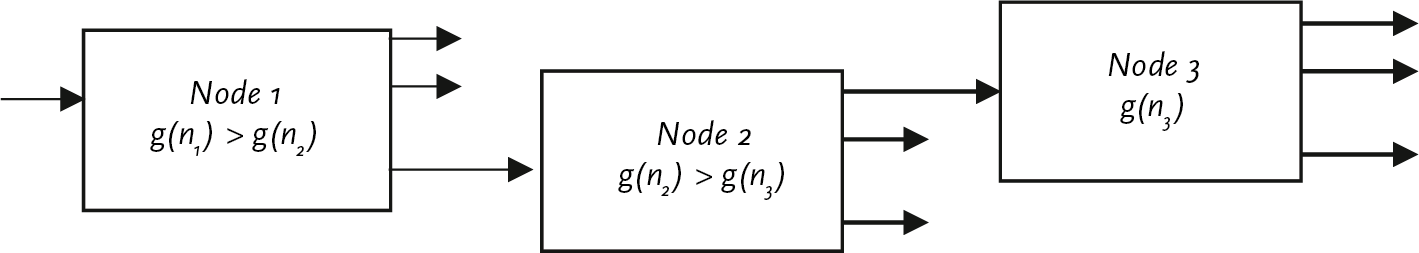
The location of the considered point affects the ‘local’ diversity. In general, closer to the supply, the local simultaneity factor will be greater than at a point further away from the supply. This is because, with a large number of loads, the random behavior is ‘averaged out.’ At a point further away, the number of connections is smaller, causing the total loads to behave more erratically. Figure 3.14 illustrates this. In node 1, the local simultaneity factor for a total of n1 connections is given by g(n1). This value is greater than the local simultaneity factor at the more distant node 2 with a total of n2 connections. The same applies to node 3. The total simultaneity factor in node 1 for all n connections is calculated from the product of all underlying simultaneity factors:
|
[ |
3.15 |
] |
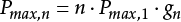
The maximum load for n equal connections is calculated from the simultaneity factor and the maximum load for one connection:

|
[ |
3.16 |
] |
where:
| n | the number of consumers |
| Pmax,1 | maximum value of the load of one connection |
| gn | simultaneity factor for n connections |
Electricity consumption is the amount of electrical energy used per unit of time, usually per year. Consumption can pertain to a single connection or to a network segment. Electrical energy consumption E is represented in kWh/year. For the various load categories, the electricity consumption per connection is generally better known than the maximum load per connection. For designing a distribution network, a relationship between consumption and maximum load is needed. One of the possibilities for this is the operating time of the maximum load. This is defined as the quotient of the annual electricity consumption and the maximum load in that year. The greater the diversity, the smaller the operating time of the maximum.

|
[ |
3.17 |
] |
To make a well-founded statement about the maximum load of a load category, Velander empirically established this relationship with consumption based on measurements in 1952. He assumed that the loads behave as mutually independent stochastic variables at a specific moment. This relationship was later used in 1975 by Strand and Axelsson for application in a computer system that manages the consumption and maximum load of a distribution network.
The Velander relationship is suitable for calculating the maximum load of load categories. In combination with load forecasting, the models of Rusck and Velander form the basis for designing medium-voltage (MV) and low-voltage (LV) networks.
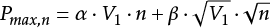
The Velander formula is as follows (Velander, 1952; Strand-Axelsson, 1975, and EnergieNed, 1996):
 |
[ |
3.18 |
] |
where:
| Pmax,n | maximum load of n connections (kW) |
| V | annual consumption of n connections (kWh/year) |
| α, β | parameters determined by measurement |
The parameters α, β and V describe the load category. These parameters depend on:
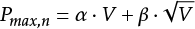
By dividing Velander’s formula (3.18) by the number of connections, the equivalent simultaneous maximum load per connection at any given location in the considered network section is obtained, where n similar connections are present.
|
[ |
3.19 |
] |
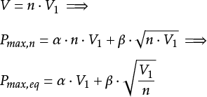
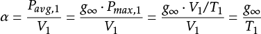
With the equivalent simultaneous maximum load per connection, the simultaneous maximum load of a network section is essentially distributed over all individual connections. The value of Pmax,eq decreases with an increasing number of connections. The less erratic behavior of the load pattern near the supply points of a network section compared to the individual connections is noticeable because in the second part of the equation, it is divided by √n. For an infinite number of connections, the equivalent simultaneous maximum load per connection is equal to α·V1. Figure 3.15 illustrates this. The graph shows two curves for a consumption of 4300 kWh/year and 2300 kWh/year. The parameters used are:
α = 0.23·10-3
β = 0.016
By considering the specific consumption of one connection, the simultaneous maximum load for n connections can be determined using the parameters α and β.

|
[ |
3.20 |
] |
By combining equation 3.20 with Rusck’s formulas (3.6 through 3.14), the following relationships are derived.

|
[ |
3.21 |
] |

|
[ |
3.22 |
] |
With these relationships, the parameters α and β can be determined if the annual consumption and the average and maximum power per connection of the connection category are known. It should be noted that the average power Pavg,1 is not equal to the annual consumption divided by the number of hours in the year. As noted in the previous paragraph, the load does not behave as a normally distributed stochastic variable over a full day. Therefore, Pavg,1 the average value of the stochastic variable that can be assumed to be normally distributed within the considered time window. This is the average value during peak load.
If for a certain type of user for one connection the annual consumption V1, the operating time T1 and the simultaneity factor for an infinite number of users g∞ are known, the parameters α and β can be determined. The maximum load for a single connection Pmax,1 follows from the definition of operating time and the average load and can, according to Rusck, be calculated from the simultaneity factor and the average load:
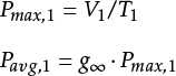
|
[ |
3.23 |
] |
The value of g∞ can, according to Rusck, be derived from the simultaneity of n users:
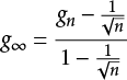
|
[ |
3.24 |
] |
By substituting these equations into the formulas that describe the relationships between Velander and Rusck, the parameters α and β can be determined.
|
[ |
3.25 |
] |

|
[ |
3.26 |
] |
Conversely, the stochastic parameters can be determined from Velander’s parameters. By combining Velander’s equation with Rusck’s formulas, the following relationships are obtained. The average value of the stochastic load is derived from:
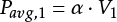
|
[ |
3.27 |
] |
The spread of the stochastic load is subsequently calculated with:
|
[ |
3.28 |
] |
An aspect such as load variation can easily be incorporated into the patterns of the averages. However, the standard deviation must always stay in line with the average value. A tool for this is the constant C. With an increase in load, without an increase in the number of connections, the standard deviation must increase proportionally.
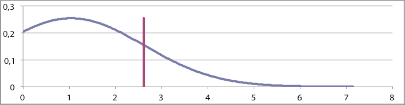
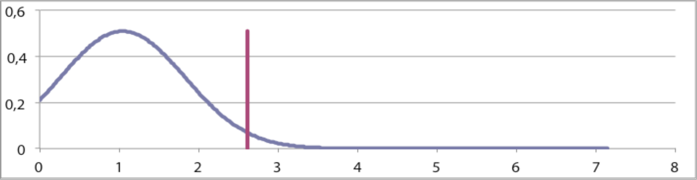
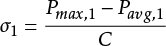
The factor C is decisive for the probability that in the model the stochastic load is greater than the maximum load Pmax. With a value for the constant C equal to 1, the maximum value of the load is determined by μ+1·σ. Due to the properties of the normal distribution, the actual maximum will be below this μ+1·σ value with approximately 85% certainty. If the constant C is taken to be 2, the actual maximum will be below this μ+2·σ value with approximately 97.5% certainty. The parameter σ1 depends on the choice of C. Above, the probability distribution is shown for C = 1, 2, and 3, respectively. In figure 3.16, the value Pmax,1 is indicated in the graphs with a vertical line. When calculating the probability distributions, the following assumptions were made:
α = 0.23·10-3
β = 0.023
V1= 4500 kWh/year
Pavg,1= α·V1= 1.04 kW
Pmax,1= α·V1+b·√V1= 2.6 kW
g∞= Pavg,1/Pmax,1= 0.4
C·σ1=Pmax,1– Pavg,1=1.54 kW
C = 3
σ1 = 0.51 kW
The graphs in figure 3.16 illustrate that the dispersion is inversely proportional to the constant C. See also figure 3.10. With a small value of C the extremes calculated with this probability distribution become larger. This must be considered when interpreting the results.
For planning, average patterns with a relatively small deviation are used. When recalculating for individual consumers, the shape of the average pattern does not change, but the associated deviation becomes relatively larger. This method does not account for individual extremes. In that case, the old method of calculating with maximum values would be more suitable.
The relationship between consumption and the maximum load of a similar group of connections is described by the Velander formula (equation 3.18). This formula uses two parameters, α and β, which are determined based on measurements. Generally, it is assumed that the measurements are sufficiently representative. Since the measurements can be considered a sample, the general rules of statistics dictate that the number of measurements (the population) must be large enough. When adding a new measurement to a collection of measurements, the parameters to be determined will generally change. As the number of measurements increases, the parameters converge to a fixed ‘real’ value. The larger the population, the better the parameters approximate the real value.
It is important to perform the measurements on several similar characteristics:
In the measurement program, the goal is to achieve a sample that is as representative as possible. This means that measurements have been conducted on both individual connections as well as on the low-voltage cables and the distribution transformer of the supply area. To this end, power meters have been placed on the connections, low-voltage cables, and distribution transformers. In an (unspecified) sample at a network company, measurements were taken on 18 individual connections with annual consumptions ranging from 1.5 to 14 MWh and on larger service areas with annual consumptions ranging from 681 to 10,170 MWh.
The parameters of the Velander formula (equation 3.18) are determined using the least squares method. This method calculates the values of the parameters α and β, for which the sum of the squared differences between measured values and calculated values is minimized. The method is based on m measurement points (x1, f1), (x2, f2), ... , (xm, fm), where xi is a measured annual consumption and f1 a measured maximum. These data points are approximated with the polynomial below.

|
[ |
3.29 |
] |
The method of least squares leads to the normal equations of Gauss. Under the condition that, in relation to Velander’s formula, the parameter a0 is equal to zero and that only the parameters are being sought a1 and a2, this leads to equation 3.30.

|
[ |
3.30 |
] |
If these equations are substituted:
a1= β
a2= α
x1= √Vi
fi= Pi
the normal equations transform into:
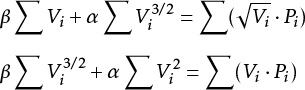
|
[ |
3.31 |
] |
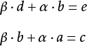
These equations can also be written as:
|
[ |
3.32 |
] |
Where:
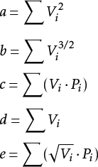
|
[ |
3.33 |
] |
These are two equations with two unknowns α and β which are easily solved. After working out the summations for all the measurements, the parameters ultimately follow α and β:
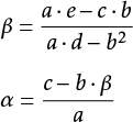 |
[ |
3.34 |
] |
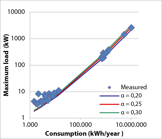
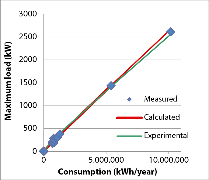
Using the above method, the sample measurements are calculated as follows: a = 0.25·10-3 and b = 0.04. Figure 3.17 shows the measurements and the curve in a single graph. The diversity of the measurements is significant. The method estimates the parameters based on the smallest sum of squared deviations. This results in measurement points with high maximum loads weighing more heavily than those with low maximum loads. This method is preferred due to the law of large numbers in statistics. However, the model must also be representative of small numbers. Plotting the data in a graph with a double logarithmic scale provides more insight into the deviations of the measurements relative to the curve.
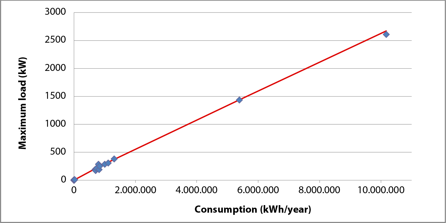
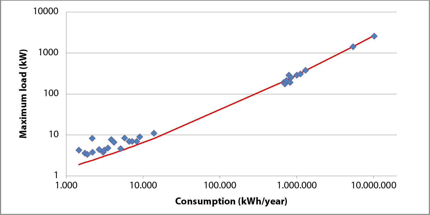
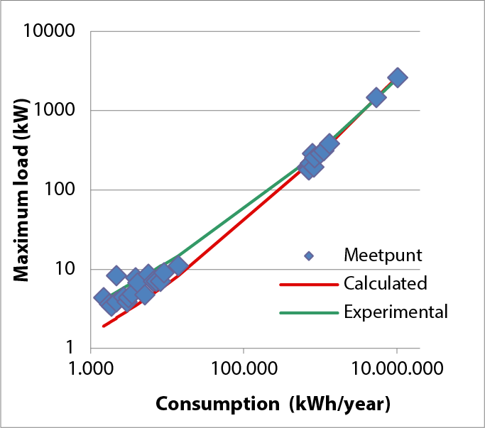
The diversity in the measurements is clearly visible in the graph. Visible are a group of measurements for small consumers, several measurements for small distribution transformers, and two measurements for large distribution transformers. A study of the graphs in Figure 3.17 and Figure 3.18 shows that the curve is a good representation of the measurements for larger loads. For the measurements in the small consumers group, the curve is not representative.
If in Velander’s formula the annual consumption of n connections is written as the product of the average annual consumption of one connection and the number of connections, it becomes:
 |
[ |
3.35 |
] |
Here it is clearly visible that the parameter α has the same influence for both small and large numbers of connections. The parameter β has through the square root of n relatively more influence for small numbers of connections.
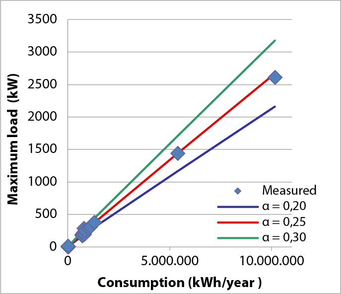
The graphs in figure 3.19 illustrate the influence of variation of the parameter α on the position of the curve relative to the data points. The first image shows the graph on a linear scale, and the second image on a double logarithmic scale. The images illustrate that variation of parameter α has a simple linear influence on the curves. For resolving discrepancies relative to measurements of low consumption and low load, variation of α does not provide the correct adjustment.
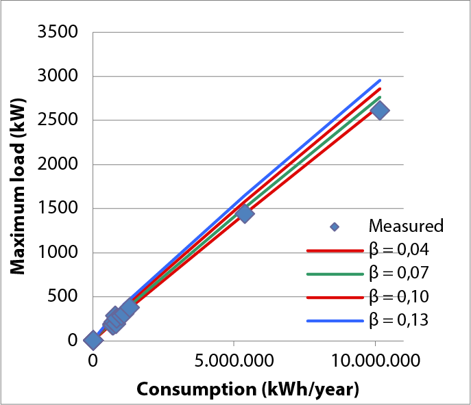
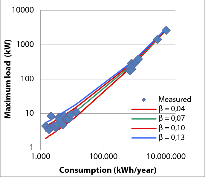
The graphs in figure 3.20 illustrate the influence of variation of the parameter β on the position of the curve relative to the data points. The first image shows the graph on a linear scale, and the second image on a double-logarithmic scale. The images illustrate that variation of parameter β has a relatively large influence, particularly at lower power levels.
In the described method, higher power levels carry more weight in the parameter determination. When considering the relative deviations from the calculated value, measurements of low consumption and low load are given more weight in the parameter determination. This method uses equation 3.36.
From Velander’s formula follows:
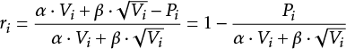
|
[ |
3.36 |
] |
where:
| Pi | measured maximum load (kW) |
| Vi | measured annual consumption (kWh) |
| α, β | to determine parameters |
| ri | residual of measurement i |
It is not easy to establish the residual equations from this formula, which means that the method of solving using Gauss’s normal equations (equations 3.29 through 3.34) cannot be applied. However, it is possible to use a computer program to vary the parameters α and β to find the smallest sum of the squares of the residuals ri determined. Using this ‘experimental method,’ the measurement data from a sample is: α = 0.20·10-3 and β = 0.09. Applying these values results in the curve being too low for high power levels. The least squares method, after all, leads to a curve where the data points have deviations both above and below. The experimental nature of this method allows for the parameters to be adjusted so that the curve does not fall too far below the measurement values for both high and low power levels. A better fit is found after adjusting the parameters: α = 0.22·10-3 and β = 0.10.
The images in figure 3.21 show in a single graph the measurement points, the curve according to the parameter determination (which favors the high power levels), and the curve according to the experimentally estimated parameters.
In the context of making society more sustainable and the ongoing energy transition, alternatives for energy use are being sought. Examples can be found in the use of electrical energy as an alternative to other energy carriers, such as electric cars and space heating using heat pumps and electric auxiliary heating. Another example is the alternative way of generating electrical energy using wind turbines, µCHP systems, and solar energy systems (PV).
A disadvantage of these developments is that they are responsible for a significant increase in electricity transport over the distribution network, accompanied by a very high simultaneity value. In networks where these new developments are applied, it is no longer sufficient to account only for the portion of the load that behaves asynchronously; consideration must also be given to a new component of the load that behaves with high simultaneity. For instance, uncontrolled, nearly all electric cars will be charged upon returning home at the end of a workday, and heat pumps with possible auxiliary heating will all be in operation simultaneously on cold days. As a result, the design of the network (both existing and new) will increasingly need to take into account the sum of the individual maximum loads.
In a growing number of new construction projects, homes are being equipped with heat pump systems for heating and cooling. Currently, 6% of new homes are being fitted with a heat pump, which corresponds to the installation of 3,500 heat pumps per year. For now, these are mainly electric heat pumps. The operating principle is similar to that of a refrigerator or air conditioner. To heat a space, heat is extracted from a medium. This medium can be the outside air or ground. The advantage of these systems is that they can work both ways. This means that a space can also be cooled by releasing heat to the same medium. When using ground or brine water as the medium, heat can be stored in the ground during the summer, which can then be extracted for heating purposes in the winter. Although these heat pump systems are more energy-efficient than traditional heating boilers, they still consume a significant amount of electrical energy. The electrical capacities range from 2 to 5 kW for an average home. Additionally, the heat pump is often equipped with an auxiliary heater with a capacity of approximately 6 kW, which can activate during low outside temperatures and after a prolonged power outage. Low outside temperatures and outages affect all homes simultaneously. Therefore, when heat pumps are widely used in homes, it must be taken into account that these devices exhibit a high degree of simultaneity in electricity demand. This demand is mainly determined by the need for heating in the winter or cooling in the summer. Particularly in the winter, the need for space heating increases simultaneously for all homes in the late afternoon and evening as it normally gets colder. Similarly, on the hottest days of summer, the need for space cooling will rise simultaneously. The actual behavior depends on the insulation level of the home. In well-insulated houses, the (24-7) electricity profile of the heat pump will be almost flat.
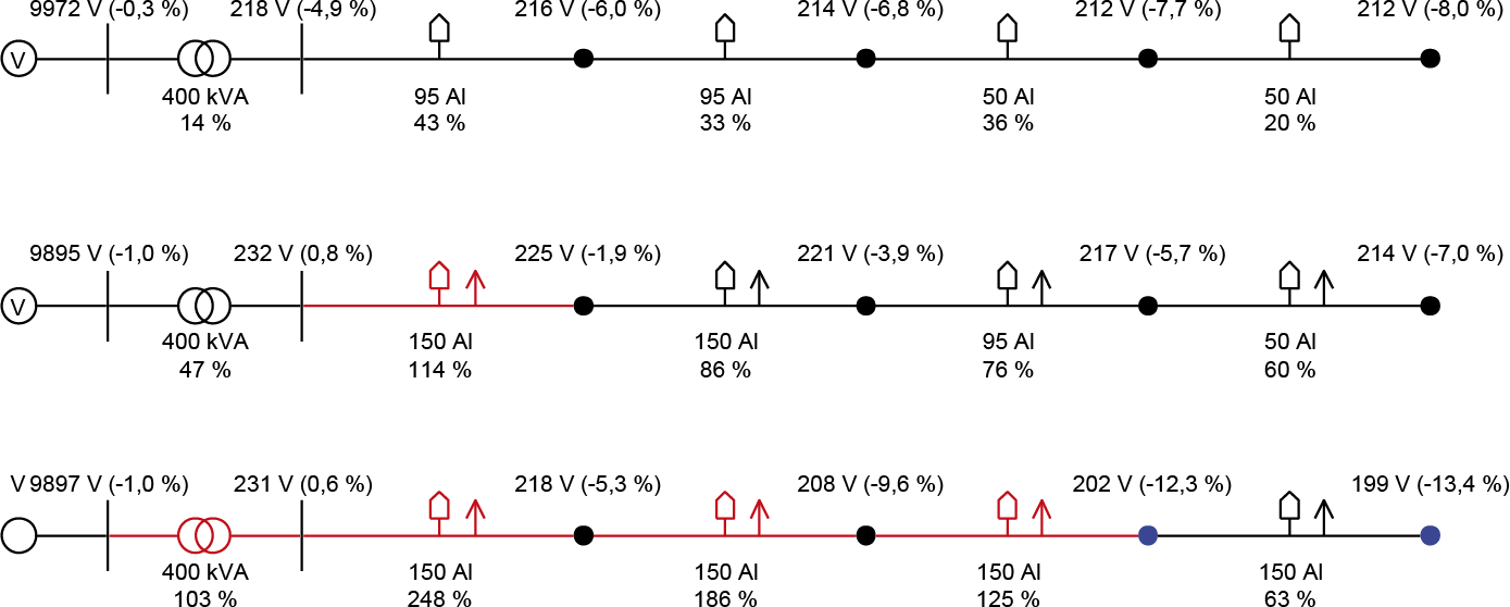
In projects where these systems are applied, the Velander method cannot be used without adjustments, and consideration must be given to the simultaneous activation of almost all heat pumps. This often includes the auxiliary heating in addition to the usual small-scale load. This means that the total load is divided into a part with high simultaneity and a part with low simultaneity. Figure 3.22 shows a section of a low-voltage network with 4 sections, each with 10 detached houses: 1) without heat pumps (top), 2) with heat pumps (middle), and 3) with heat pumps and activated auxiliary heating (bottom). In the calculation of the LV supply cables, a power of 3 kW per heat pump and 6 kW per auxiliary heating was assumed. In the case without heat pumps, the LV main cable with aluminum conductors can be reduced from 95 to 50 mm2 conductor cross-section. In the case with only heat pumps, cables with a 150 mm2 conductor cross-section are used in the first two sections and even then the first section is overloaded. In the case with heat pumps and activated auxiliary heating, the network with the application of 150 mm2 aluminum cables is heavily overloaded and the voltage at the end of the line is too low. A solution to this problem can be found by allowing fewer connections on a line or by working with parallel cables, assuming that no cables with a larger conductor cross-section are used.
If the heat pump and auxiliary heating are connected in three phases, this results in an additional load per connection of 9000 kVA / 3 / 235 V = 12.8 A per phase. With a simultaneity factor of 1, this can simply be multiplied by 10 for 10 connections, resulting in an additional load current of 128 A. This current is added to the standard load of 10 detached houses, which is a maximum of 24 A, resulting in a total load current of 128 + 24 = 152 A, as seen in the last cable section of figure 3.22. This shows that the impact of heat pump systems (128 A) is so significant that the influence of the stochastic behavior of the remaining load (24 A) can be practically neglected.
The electric car began a slow rise in 2010. In the event of a breakthrough, there are concerns that peak load will increase abruptly. The forecasts for the number of electric cars in the Netherlands in the year 2020 vary widely, from 200,000 to more than 1 million. A quarter of a million is already ambitious but theoretically achievable. The effect of this will be most noticeable in the low-voltage networks, immediately followed by the medium-voltage networks. In this context, the network operator faces several uncertainties. Among others: how can this new development be properly integrated with the existing electrical transport capacity, and how should newly designed networks be prepared for this? To answer these questions, the expected electrical behavior of the electric car must first be examined.
In 2007, a passenger car drove an average of 13,877 km per year (CBS). It is assumed that the consumption of the electric car is 5-7 km/kWh (an average of 1 kWh per 6 km). This is based on specifications from suppliers and on practical figures, which range from 1 per 4 to 1 per 7, depending on driving style and type of car. This means that the annual consumption of an electric car is equal to 13,877/6 = 2,312 kWh/year. Based on this annual consumption, this amounts to a consumption of approximately 6.3 kWh per day. For comparison, the average annual consumption of a household in 2007 is 3,512 kWh (9.6 kWh per day).
The peak load of an electric car is determined by the amount of energy to be recharged and the duration of the charging. For calculating the peak load in a home situation, it can be assumed that an empty battery should be able to be charged overnight. Assuming a duration of 8 hours (from 11:00 PM to 7:00 AM) and a battery capacity in the car of 16 to 36 kWh (as of 2009; 100 kWh in 2025), the required charging power of a car is:
There are electric cars whose peak charging power is adjusted to a regular installation of 10 A and 230 V, limiting the peak charging power to 2.3 kW. There are also electric cars equipped with a three-phase plug, suitable for 3*16 A (32 A in 2025) and 400 V. With this, charging with one phase can be done at 3.5 kW and with three phases at 11/22 kW. The European standard plug (type 2) is suitable for 3 x 63 A and 400 V. This would correspond to a peak charging power of 40 kW. This capacity is not yet fully utilized for home charging points. As of 2010, the development of chargers has not progressed that far. Some manufacturers are considering an on-board 20 kW charger. If such chargers are allowed to charg in large quantities and charged simultaneously, they will pose a problem regarding the peak load on the distribution network in home area’s.
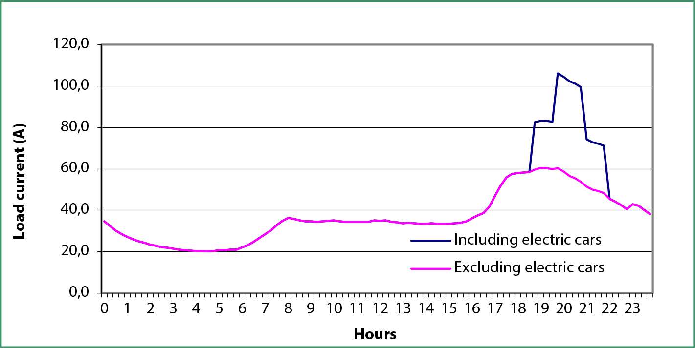
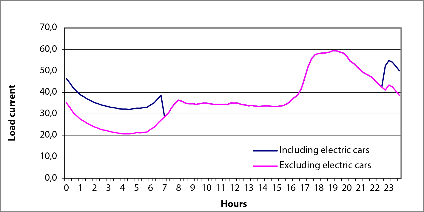
A power of 4.5 kW for charging a large battery in 8 hours can no longer be supplied by a regular outlet with a single 16 A fuse. In that case, a three-phase connection must be used, or a longer charging time must be accepted. A duration of 10 hours means a charging power of 3.6 kW, which corresponds to a current of 15.7 A at a voltage of 230 V. A condition is that the charging cycle for each electric car, regardless of the battery’s state of charge, is spread over the maximum duration of 8 to 10 hours. It should be considered that in many household situations, the charging time could also be 12 hours, which could reduce the peak load. Figure 3.23 illustrates the electricity demand in the case of an uncontrolled charging cycle, where the current is very high for a short period in the evening. Figure 3.24 shows a situation of an optimized charging cycle, where the duration is set by the customer. The example assumes a neighborhood with 40 single-family homes, of which 25% need to charge an electric car. Thus, in this example network, there are 10 electric cars, with an average energy requirement of 6.3 kWh per day.
With an uncontrolled charging cycle, an average energy of 6.3 kWh per car can be delivered in 2 hours at a current of 13.7 A and a single-phase voltage of 230 V. In the example, it is assumed that half of the cars start charging at 7:00 PM and the other half at 8:00 PM. This causes an additional current of 23 A per phase in the first hour and an additional current of 46 A per phase in the second hour. If this occurs during the evening hours at peak load times, the grid can become overloaded.
With a controlled and optimized charging cycle, the average energy of 6.3 kWh per car can be delivered over 8 hours at a current of 3.4 A and a single-phase voltage of 230 V. In the example, it is assumed that all cars start charging from 10:00 PM. This causes an additional current demand of 11.4 A per phase on the grid.
For more information, see https://elaad.nl/en/topics/smart-charging/
The above example illustrates the importance of spreading out the charging period of electric cars. Load management also prevents charging from starting before or during the peak evening hours.
By charging the batteries in a controlled manner (smart charging), the demand is adjusted to the grid capacity and potentially to the supply of sustainable energy. The currents at which batteries are charged when connected to the grid may vary during the charging session. In this process, the batteries are only charged from the grid. The batteries can, in principle, also be used as a buffer for the grid, where they supply electricity back to the grid. This will increase the number of charge and discharge cycles. A disadvantage of this is that it can lead to faster wear and tear on the batteries. Therefore, this will only be applied in moderation.
Experiments are being conducted with fast charging within 20 to 40 minutes. In practice, fast charging means charging the battery from 20% to 80% capacity, not from 0 to 100%. However, due to the high power involved, significant heat loss occurs. Therefore, the charging power quickly becomes 10% or more greater than the power that actually goes into the battery. For charging 60% within half an hour, the required charging power per car, including heat losses, is:
These power levels correspond to an LV three-phase system with a current of 30 and 70 A, respectively, assuming a power factor of 1. Establishing a facility to fast-charge multiple cars requires a specific investment in the infrastructure. Due to the high current demand that occurs in this scenario, this may potentially lead to the need for a dedicated MV connection or a distribution station.
For calculating the simultaneity of charging many cars in a residential situation, one can assume an average electricity consumption of 6.3 kWh/day per car. The simultaneous load on the grid by charging at night for 8 hours would then be 6.3 kWh divided by 8 = 0.79 kW per electric car (based on data from an electric car in 2010). The problem with simultaneity is that there is no experience yet with large-scale charging of electric cars. In the worst case, the simultaneity factor is 1, meaning all peak charging capacities are connected simultaneously. This means that the additional peak load can range between 0.79 kW per car and 10 kW per car, based on the technology applied in 2010.
Calculating with simultaneity always assumes large numbers. The number of electric cars is still small. Moreover, the diversity of charging needs is significant. Additionally, consideration can be given to the possibility of charging car batteries during the day, in parking lots at shopping centers or at work. Specifically, the large number of electric cars can lead to a significant, previously unforeseen increase in the local load on the network.
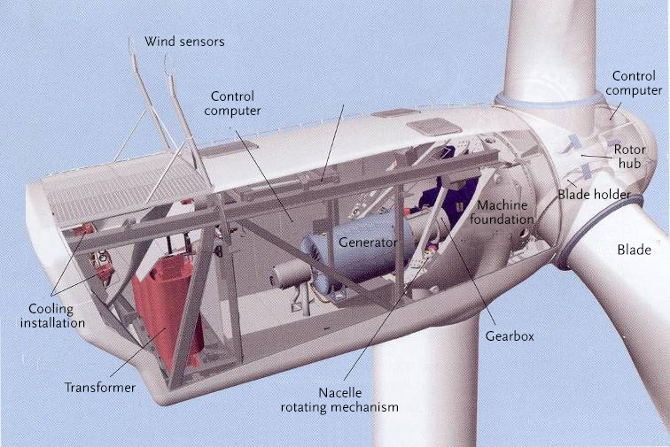
Decentralized generation is no longer a marginal phenomenon in distribution networks. The systems used range from µCHP units and PV systems in low-voltage networks to large CHP and wind energy systems connected to medium-voltage and high-voltage grids. On land, wind turbines with capacities of 3 to 5 MW each (offshore 16MW – 2025), grouped in wind farms, feed into transmission networks at medium-voltage or high-voltage levels. In combined heat and power plants, large generators are used, which, depending on their capacity, are connected to either the distribution or transmission network. Additionally, large numbers of small generators, such as those in µCHP installations, are increasingly being used in low-voltage networks. These are usually connected via converters.
Various definitions for decentralized generation are used in the literature. Most definitions are based on the type of technology applied, the environmental impact of the installation, the size of the installed capacity of the installation, and the voltage level to which the installation is connected. A definition based on the type of technology is challenging due to the wide variety of technological developments, such as CHP systems, PV systems, and wind turbines. A definition based on the voltage level or the size of the installed capacity is also used. The NMa does not use a specific definition of decentralized generation, but refers to:
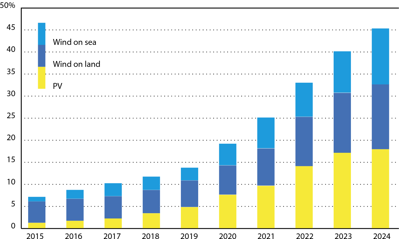
Additionally, the NMa uses the term ‘sustainable electricity,’ which is generated from renewable energy sources such as wind, solar energy, geothermal energy, wave energy, tidal energy, hydropower, biomass, landfill gas, sewage treatment gas, and biogas (Electricity Act 1998). A large portion of decentralized generation falls under the category of sustainable electricity. The production of sustainable electricity increased from 6.0 percent of domestic electricity consumption in 2007 to 7.5 percent in 2024. This increase is due to a rise in electricity production from wind energy and biomass.
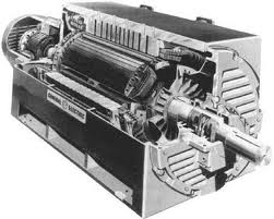
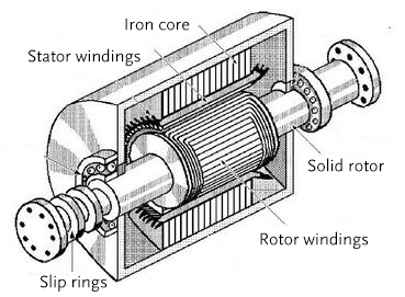
The generators of decentralized producers are usually designed as synchronous machines and sometimes as asynchronous machines. A synchronous generator has a rotor that is energized in such a way that it behaves like a rotating magnet. The rotor rotates in the electromagnetic field generated by the stator windings that are connected to the power grid. As a result, the synchronous machine is forced to rotate in sync with the rotating field determined by the grid. The frequency of the voltage generated by the synchronous generator must be 50 Hz. An asynchronous generator, on the other hand, has a short-circuited rotor winding, in which a current flows whose magnitude and frequency depend on the difference in rotational speed of the rotor relative to the rotating electromagnetic field of the stator windings. The asynchronous generator can only generate power if it rotates (4 .. 6%) faster (thus asynchronously) than the rotating field determined by the grid.
Decentralized generation affects the behavior of currents and voltages in the distribution network. In general, a generator causes an increase in voltage and an increase in short-circuit power. Sometimes this can be desirable, but sometimes not. A power flow and short-circuit calculation provides more insight into this. This is further discussed in chapters 9 and 10. The maximum short-circuit current of generators connected via converters is limited by the electronics to approximately the nominal current. The following systems are most commonly used in distribution networks and medium-voltage transport networks.
Larger wind turbines with a capacity of 5 MW or more and large CHP systems cannot be integrated into the grid without further consideration. A detailed study and calculation of the effects associated with supplying or not supplying electrical energy to the grid, as well as the consequences of a short circuit in the grid, must be conducted in advance.
In a growing number of new construction projects, homes are being equipped with µCHP systems. These systems can deliver a relatively small power output of 1 to 5 kW per connection. The simultaneity of these systems is quite high. After all, electricity production follows the heat demand, which depends on the residents’ patterns. In a relatively large group of similar homes, it can be expected that the heat demand will also be similar on average. For example, most working people will come home around 6:00 PM, and during cold days, the heat demand in homes will increase at that time. For non-working people, the heat demand will vary less throughout the day. The advantage of this form of decentralized generation is that most electricity production largely coincides with the demand. Especially in the winter months, the normal load of residential areas in the evening hours is quite high, as illustrated in figure 3.4. As a result, the net load on a distribution network will decrease due to the µCHP systems. However, the behavior of the connected users is uncertain, so for reducing the peak, an estimate of the minimum output of the µCHP systems can be used.
In low-voltage networks, single-phase µCHP systems are used. These are relatively simple components for network calculations, exhibiting specific behavior during startup and in case of short circuits. In particular, the collective behavior during short circuits and the simultaneous startup after the restoration of the power supply is a subject of study in (future) projects.
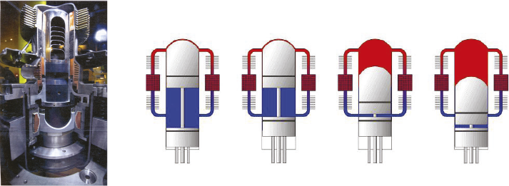
Many µCHP units are equipped with a Stirling engine. In a Stirling machine, the combustion of the fuel takes place outside the engine. The working medium, such as air or helium, that is inside the machine never leaves it. The engine consists of a cold part and a hot part. These are indicated in figure 3.27 with blue and red. A heat source, such as the flame of a gas burner or hot gases from a heating boiler, continuously heats the hot part of the engine while the cold part is continuously cooled by, for example, the return circuit of the heating system. Both parts, hot and cold, are constantly connected to each other. The working medium is moved back and forth between the hot and cold spaces by a displacer (almost) without work, where the medium in the hot space expands by absorbing heat and performs work by moving a piston. The air is then moved by the displacer back to the cold space, cools down there, and decreases in volume. The working medium, confined within the engine, thus continuously circulates from the hot part to the cold part and vice versa, moving the piston back and forth. The piston can drive a linear generator or, via a transmission, a more conventional rotary generator.
There are two variants for electricity generation in µCHP systems.
This generator is not a rotating machine. The electrical power is generated by a linearly oscillating magnet, which is driven by the piston of the Stirling engine. The generator is connected to the grid via a converter.
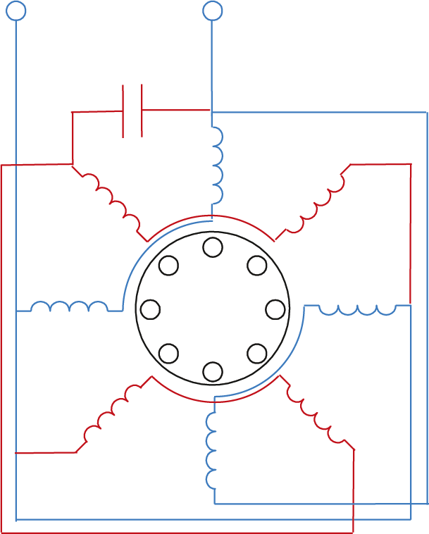
The WhisperGen-CHP uses a modified asynchronous generator that is driven by four pistons of the Stirling engine via a transmission. The stator of the small asynchronous motor is wound as a 4-pole two-phase generator. The current in the auxiliary winding is shifted by 90 degrees using a capacitor to generate a rotating magnetic field. Figure 3.28 illustrates this with the winding diagram for the stator. The main winding is indicated in blue and the auxiliary winding in red.
Sunlight is converted into direct current by photovoltaic cells in solar panels. Through a converter, the solar panels are connected to the grid for power transfer. As of 2025, solar panels have a power output up to 1000 W/m2 . Practically, this leads to power outputs of 4 kW peak power per connection (with 10 panels). Figure 3.29 shows a PV system with 112 280 W-panels. Together, these 112 panels are good for over 30 kW (from a 63 kW farm). With large-scale application, these PV systems can produce so much electricity on summer days that during periods of low demand, the energy demand turns into an energy surplus, causing the energy flow direction in an LV network to reverse.
The simultaneity of electricity yield from PV systems in an LV distribution network is high, due to the ratio of the area affected by cloud cover to the size of the area served by a secondary substation. A PV simultaneity factor of 1 can safely be used for planning LV distribution networks if all panels are facing south. The service area of a substation covers a much larger area, reducing the simultaneity of all PV systems in case of cloud cover. However, on a clear day, all PV systems will produce at maximum capacity, so a simultaneity factor of 1 can also be used on the scale of an MV distribution network. Studies on the impacts of PV systems will mainly focus on local LV distribution networks. These studies will particularly look at the combination of maximum yield and minimum load.

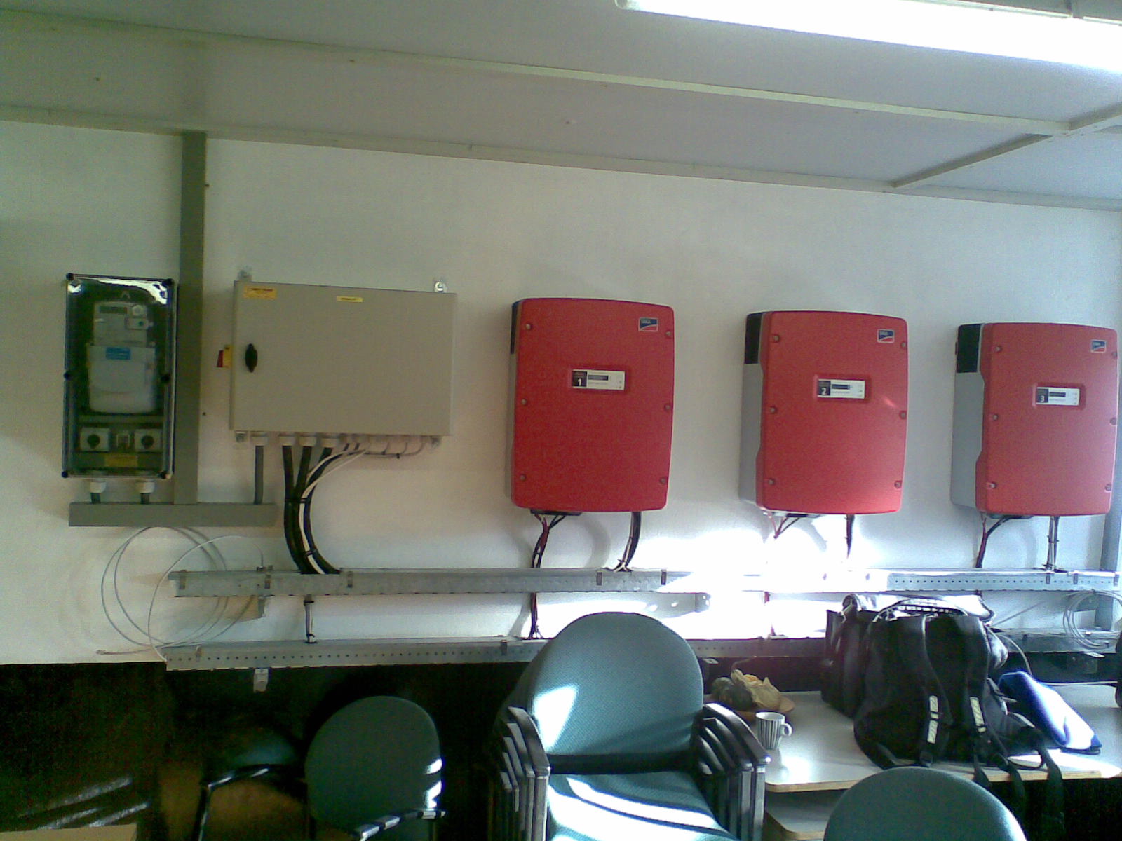
The PV systems are always connected via an inverter. Figure 3.30 shows a system with three converters for a total power of 30 kW. The PV panels provide a direct current voltage of approximately 40 V each, which needs to be converted. As a result, the short-circuit power is always limited to the maximum nominal current of the inverters. A PV system only delivers power when the system is connected to the 230 V distribution network. In case of a malfunction, the converter stops production. This is a safety requirement.
Wind turbines have a nominal capacity of 1 to 5 MW per turbine. They are usually clustered in wind farms, ranging from small to fairly large groups. In the past, these wind farms were only placed on land, but increasingly, large wind farms are being built offshore. The potential yield of offshore wind energy is estimated to be twice the total Dutch energy consumption.
The power of a single wind turbine is too large to be connected to a low-voltage 400 V grid (800 A at 690 V). A power of 1 MW already results in a current of 1.4 kA in an LV grid. For this reason, wind turbines are connected at the MV level. Large wind farms are connected at the HV or HV-DC level.
There are wind turbines for constant and variable rotational speeds. In wind turbines with a fixed rotational speed, the generator (an asynchronous machine) is directly connected to the grid. In these wind turbines, any fluctuation in wind speed is directly noticeable in the active power. Wind turbines with a variable rotational speed are controlled using power electronics, allowing fluctuations in wind speed to be largely stored in the rotational energy of the rotor. This ensures that wind turbines with variable rotational speed exhibit minimal fluctuations in the delivered energy.
The new large wind turbines are usually of the DFIG (Doubly Fed Induction Generator) type, with the stator winding directly connected to the grid and the rotor winding connected via a converter. By varying the frequency of the current through the rotor winding, this synchronous generator can operate at variable rotational speeds. This type of wind turbine and its behavior is well described in the literature (Slootweg, 2003). These generators are used in wind turbines with capacities between 1 and 5 MW. Other mew large wind turbines are full-inverter type wind turbines.
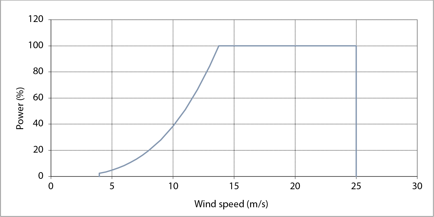
To determine the expected electricity production, understanding the power characteristic is important. The power characteristic of each wind turbine is such that below the cut-in wind speed, the power is zero. Above this wind speed, the electrical power depends on the cube of the wind speed. Above the nominal wind speed, the power is constant and equal to the nominal power. Above the cut-out wind speed, the wind turbine is reduced/taken out of operation to prevent damage.
A CHP system is installed to produce heat, usually at a high temperature. This heat is used in industry, for space heating, in greenhouses, or for district heating. The CHP produces steam or hot water for this purpose, and the heat is also used to generate electricity, which can potentially be fed back into the grid. The combined generation in the CHP system can achieve a high-energy efficiency.
Since 2006, electricity production in greenhouse horticulture has increased significantly. Many greenhouse horticulture companies use a gas engine to generate electricity and heat. They use this to light and heat their greenhouses. When energy prices are high, selling electricity is an attractive additional source of income for these growers. As a result, many new gas engines have been installed, doubling the electrical capacity in this sector within two years. At the beginning of 2008, more than 10 percent of the total electrical capacity in the Netherlands consisted of production units in greenhouse horticulture (CBS, 2009). This percentage has since decreased due to the increase in conventional power plants and CHP plants.
Due to the increase in the amount of decentralized generation with large CHP installations, the load on the medium-voltage distribution network can change significantly. The consequences are highly dependent on the specific location in the network. It is possible that the distribution network is not designed for a lot of decentralized input. The direction of the power flow, traditionally from a high to a low-voltage level, can reverse. This can lead to either reduced or increased network costs. Network losses can increase because the distance from the generation installation to the consumer can increase, for example, if many generators are set up in a peripheral region. On the other hand, network losses can decrease because the electrical power is generated closer to the consumer.
The electrical capacities of CHP installations range from 0.1 to 20 MW per connection. Larger capacities also exist. A 10 kV cable with an aluminum conductor of 240 mm2 may be loaded with 6 MVA. A capacity of 20 MW is therefore too much to connect to the medium-voltage distribution network. Figures 3.6 and 3.7 illustrate measurements of power flows of 20 kV lines in greenhouse areas. The patterns show daily load fluctuations up to 17 MW between maximum demand and supply. These fluctuations are caused by the sum of the patterns of the load and the generation. Particularly in greenhouse horticulture, CHP units with capacities of 3 to 4 MW are clustered. In horticultural areas, clusters with capacities up to 100 MW are connected to the high-voltage network. The size of a complete installation is then partly determined by the size of the respective greenhouse area.
Growers not only produce electricity to meet their own heat, electricity and CO2 needs, but also according to market demand for electrical energy. When the kWh price is high, they can produce extra electricity, and when the kWh price is low, they can even purchase electricity. It is more of an economic consideration than an energy-technical one. Therefore, the maximum electricity production does not necessarily coincide with the maximum local electricity demand. For connecting such large installations, a thorough study must always be conducted, considering extreme situations of maximum generation coinciding with minimum load and minimum generation coinciding with maximum load. The capacity of the medium-voltage network is limited, so often a network upgrade is necessary to connect a large cluster. In extreme cases, even an upgrade of the high-voltage network is required.
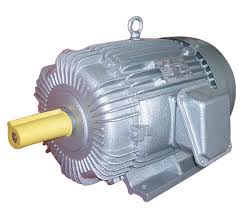
Motors are frequently used in industry and constitute the majority (~75%) of the load. When designing industrial networks, the behavior of the motors must be carefully considered. The influence of the motor is particularly noticeable when starting the motor and when a short circuit occurs in the network. Starting a motor briefly requires a large current, 4 to 8 times the nominal current, which leads to a voltage dip. This inrush current can be limited by using a star-delta connection, a soft starter, or a frequency converter. If a motor is controlled using power electronics, this can lead to an increase in the harmonic distortion of the alternating voltage. If a short circuit occurs in the network, the motors will contribute to the short-circuit current, thereby increasing it at the short-circuit location and blinding the Icc upstream. The influence of motors is minimal in most distribution networks. However, in an industrial environment where many large motors are used, it may be necessary to further study their impact on the network (expecially for IE4 motors).
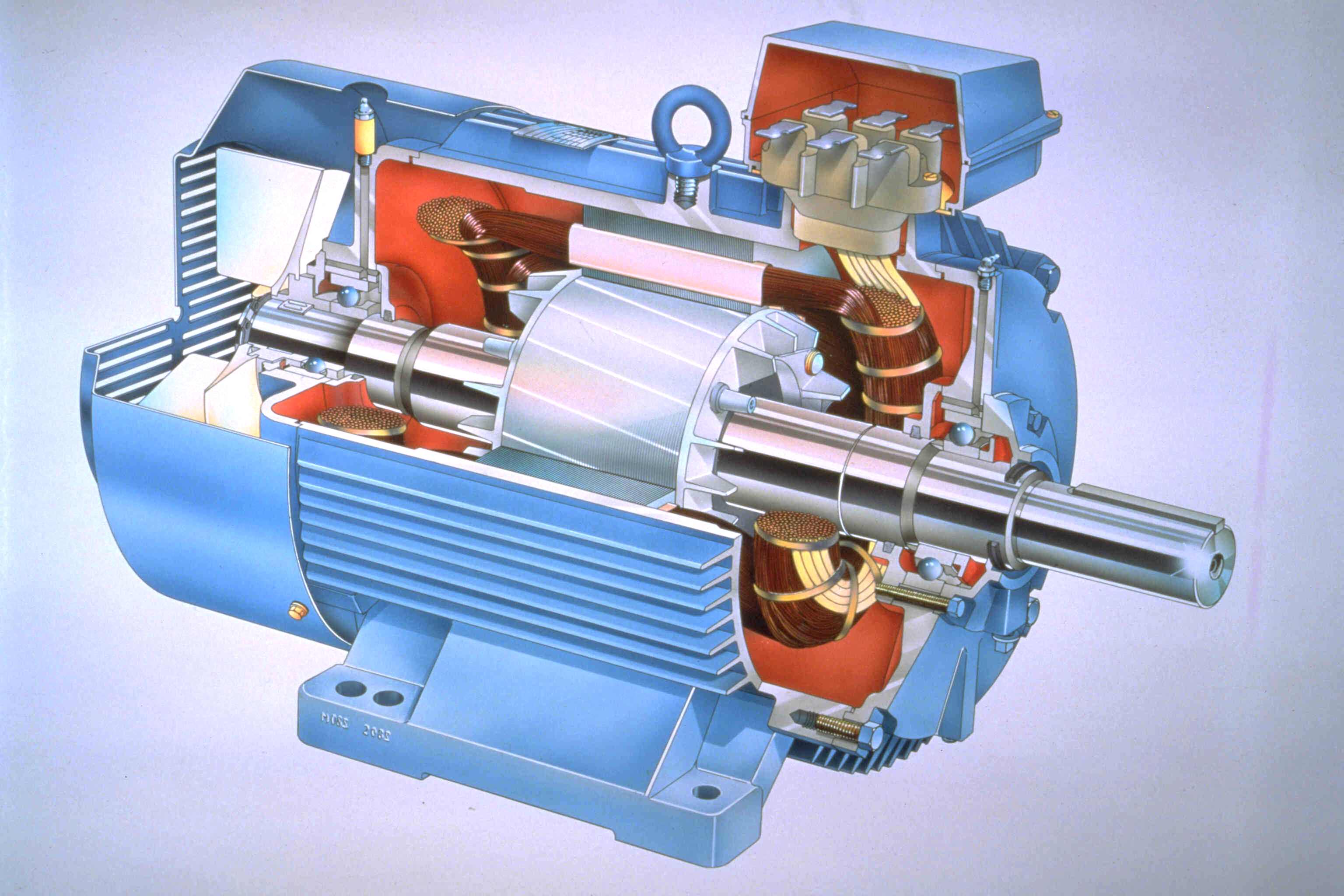
Alternating current motors exist in the forms of synchronous and asynchronous machines. The synchronous motor has the same construction as the synchronous generator. Large synchronous motors are almost exclusively used in industry. The asynchronous motor has a squirrel-cage rotor winding. These motors are also known as induction motors or squirrel-cage motors. At no load, the asynchronous motor runs slightly slower than the synchronous speed. If the motor is loaded, it will run even slower. This behavior is depicted in the torque-speed curve of the motor. As the load increases, the motor will reach a point where it can no longer deliver the required torque. The motor will then come to a stop. The point at which this occurs is referred to as the pull-out torque. When stopped, the motor will draw a current equal to the starting current.
Motors can be connected directly to the grid (DOL, Direct-On-Line). In that case, the highest starting current must be taken into account. To limit the starting current, the windings in some designs can be temporarily switched from delta to star. In this configuration, the windings receive a voltage during startup that is a factor of √3 lower than normal. Motors can also start using a soft starter. This limits the starting current to approximately the nominal current, but depends on the needed starting torque. Motors with adjustable speed are connected to the grid via a frequency converter. These converters limit the starting current to approximately the nominal current.
Asynchronous motors provide a brief contribution to the short-circuit current in the event of a short circuit in the grid, which is approximately equal to the starting current. Motors connected via a frequency converter generally do not contribute to the short-circuit current. If the frequency converter allows for feedback, the short-circuit current contribution is limited to approximately the nominal current.
|
Motor control |
Starting Current |
Contribution to the short-circuit current |
|
Directly on the grid |
6 .. 8 x nominal current |
6 .. 8 x nominal current |
|
Softstarter |
approximately nominal current |
6 .. 8 x nominal current |
|
Converter |
approximately nominal current |
no contribution or approximately nominal current |
At the low-voltage level, the networks are usually characterized by large numbers of small consumers. It is generally justified to refer to them as consumers because they primarily consume electricity. The supply areas at the LV level are typically such that the consumers have a predictable and similar character. Therefore, it is common to work with specific load types and to utilize the simultaneity of the consumers. Even if the users generate electricity themselves using, for example, PV systems, it is still justified to work in this manner.
With the introduction of large electricity consumers, such as electric cars and space heating using heat pumps and electric auxiliary heating, it is no longer sufficient to consider the non-simultaneity of the electricity demand of all consumers. Instead, it is necessary to account for the fact that large electricity consumers are operating simultaneously. Regarding future developments, the uncertainties are greatest in low-voltage networks. As a result, more and more new networks will be designed based on the sum of individual maximum loads. Consequently, network designers increasingly tend to hedge against these future uncertainties by designing the low-voltage network as robustly as possible: with maximum cable cross-sections, for example, 150 mm2aluminum conductor, and the largest possible distribution transformer, for example, 630 kVA. Additionally, the network designer will claim extra capacity in new constructions to accommodate necessary additional future network components, to avoid future costs as much as possible.
At the MV level, it must be carefully considered whether the network serves connections that exhibit abnormal behavior. In addition to the secondary substations that serve large groups of low-voltage customers, there are also small numbers of high-capacity connections that show varying load patterns over time. Specifically, decentralized generation at the MV level exhibits behavior that cannot be easily modeled with simultaneity factors. If the load behavior of a large customer’s generation is well known, load patterns can be used. In such cases, the focus is more specifically on the load and generation over a certain period. The network must then be suitable for distributing power in all situations. If the behavior is unknown and cannot be reliably determined, it is only possible to account for extreme situations in generation and load. In that case, when analyzing the MV network concerning these customers, one must assume maximum load and minimum production, and minimum load and maximum production, of course in combination with the other loads in the network.
Phase to Phase, a subsidiary of Technolution. © 2009-2025