Part 2 begins in Chapter 7 with a brief explanation of some important basic concepts necessary for calculations in electrical networks. The foundation is laid with the description of the alternating current (AC) system and the application of complex calculation methods. Next, the symmetrical components method, which is crucial for performing short-circuit calculations, is explained.
The translation of ‘Networks for Electricity Distribution’ was created with the help of artificial intelligence and carefully reviewed by subject-matter experts. Even with our combined efforts, a few inaccuracies may still remain. If you notice anything that could be improved, we’d love to hear from you.
Network calculations often make use of equivalent circuits for loads and electrical machines. An electrical machine can be either a motor or a generator. A motor draws electrical energy from the grid, while a generator supplies electrical energy. To avoid ambiguity, it is essential to define the positive direction for current, voltage, and power. This is determined by the chosen sign convention: either the motor convention (also known as the load convention or passive sign convention) or the generator convention. Figure 7.1 illustrates this for a load or motor and a generator connected to a network. The drawing convention is characterised by:
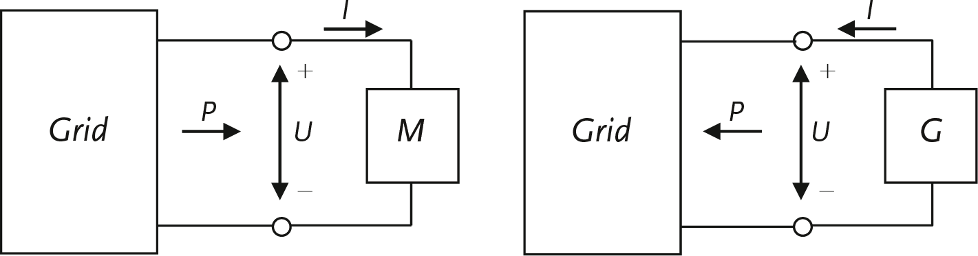
In the motor convention, he current flows from the network to the device and the sign is positive if the connected device is purely resistive. The power consumed is also positive. In the generator convention, the sign of the current is negative. The power delivered to the network is therefore negative.
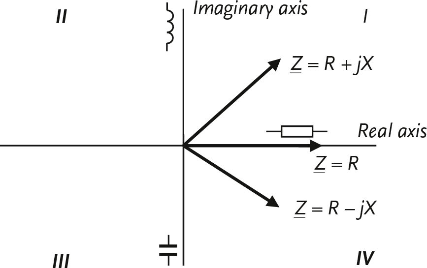
Voltage, current, and component impedances can all be represented as phasors in the complex plane. The impedance of a pure resistor is then represented by a vector on the positive real axis, whereas the impedance of a pure inductor without resistance is represented by a vector along the positive imaginary axis. The impedance of a pure capacitor is represented by a vector along the negative imaginary axis. All physical components have a positive resistance and a positive or negative reactance. As a result, their impedances are represented in the quadrants I and IV in the right plane of Figure 7.2. A load in quadrant I is called inductive, and a load in quadrant IV capacitive.
A generator is usually not modeled with an impedance. Therefore, in the same plane, active power and reactive power (apparent power) are also depicted. In the complex plane, the four quadrants are used for this purpose. The properties for the motor and generator conventions are summarized in Table 7.1.
Quadrant |
Motor convention |
Generator convention |
||
P |
Q |
P |
Q |
|
I |
> 0 (consumption, motor) |
> 0 (consumption, coil) |
> 0 (generation, generator) |
> 0 (generation, capacitor) |
II |
< 0 (generation, generator) |
> 0 (consumption, coil) |
< 0 (consumption, motor) |
> 0 (generation, capacitor) |
III |
< 0 (generation, generator) |
< 0 (generation, capacitor) |
< 0 (consumption, motor) |
< 0 (consumption, coil) |
IV |
> 0 (consumption, motor) |
< 0 (generation, capacitor) |
> 0 (generation, generator) |
< 0 (consumption, coil) |
For consistency in network calculations, it is important to choose either the motor or generator convention and apply it consistently throughout.
To clarify the relationship, the following example is given. The active power and the reactive power in the motor convention generated by a synchronous generator in quadrant III, is consumed by a motor in quadrant I.
A synchronous machine can operate both as a motor or as a generator and can absorb and supply reactive power. This machine is therefore capable of operating in all quadrants. However, it remains important to choose either the motor convention or the generator convention for each operating point once.
An asynchronous machine can also operate both as a motor and as a generator, but it can only absorb reactive power. In the motor convention, the asynchronous machine can then operate in the quadrants I and II.
Power |
Motor convention |
Generator convention |
Current and voltage angle |
Diagram |
||
Ppositive |
absorb active power |
deliver active power |
||||
Pnegative |
deliver active power |
absorb active power |
||||
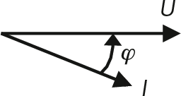
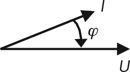
Q positive |
absorb reactive power (inductive load) |
deliver reactive power (overexcited generator) |
lagging current angle φ positive |
 |
||
Qnegative |
deliver reactive power (capacitive load) |
absorb reactive power (underexcited generator) |
leading current angle φ negative |
 |
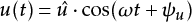
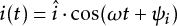
In principle, an alternating voltage can have any arbitrary waveform, as long as it repeats itself periodically. The period during which the shape repeats determines the frequency f, which is equal to the inverse of the period duration. Due to this property, the alternating voltage can be described with a function of time. The result of this function is the instantaneous value of the voltage. In almost all electricity systems, the alternating voltage is sinusoidal. It is customary to describe this alternating voltage with the following cosine function:
 |
[ |
7.1 |
] |
in which:
| û = √2·URMS | peak value of the voltage |
| ω = 2π f | network angular frequency (rad/s) |
| ψu | voltage phase angle (rad) |
The frequency is expressed in angular frequency, in radians per second. The phase angle is expressed in radians by multiplying the angle in degrees by 2π/360.
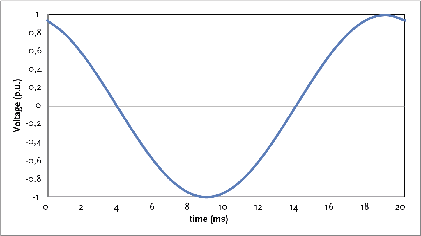
The instantaneous voltage in expression 7.1 describes the varying value of the voltage as a cosine function of time. In figure 7.3, this function is plotted, with the phase shifted by 20 degrees as an example.
The current can also be mathematically described in a similar manner. The current often has a different phase angle and magnitude than the voltage. This is caused by the properties of the components in the network and Ohm’s law. The angle of the current is expressed using the current phase angle ψi. The instantaneous value of the current is then:
 |
[ |
7.2 |
] |
where:
| î = √2·IRMS | peak value of the current |
| ω = 2π f | network angular frequency (rad/s) |
| ψi | voltage phase angle (rad) |
The phase difference between current and voltage is:
 |
[ |
7.3 |
] |
As a result, the current phase angle can also be written as:
 |
[ |
7.4 |
] |
which transforms equation 7.2 into:
 |
[ |
7.5 |
] |
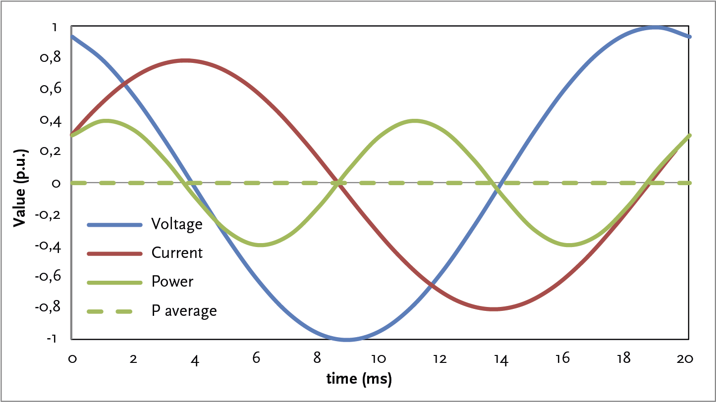
From the functions of the instantaneous value of current and voltage, the function for the instantaneous value of power can be derived by taking the product of the instantaneous voltage and current.
 |
[ |
7.6 |
] |
By using the general trigonometric relationships, it follows from equation 7.6:
 |
[ |
7.7 |
] |
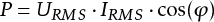
This equation can be split into two parts. It is notable that in the first part, the well-known cos(φ) appears, which is also referred to as the ‘power factor’. The first part of the equation is time-independent and is called the average power. The second part of the equation is time-dependent and oscillates at twice the frequency.
 |
[ |
7.8 |
] |
When considering the power through a pure resistor, the current is purely resistive, and the phase angle between current and voltage is φ = 0 rad. In that case, equation 7.7 simplifies to:
 |
[ |
7.9 |
] |
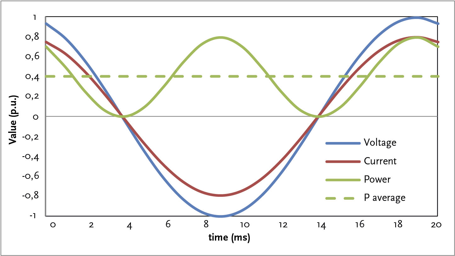
Figure 7.4 illustrates this. Here, it is clearly visible that the instantaneous power is always positive and oscillates at double the frequency around the average power (Paverage) of approximately 0.4 p.u. The average power is the power with which work is performed.
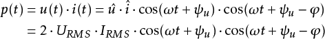
The following example assumes an impedance where the current lags the voltage by 45 degrees. According to Table 7.2, this is an inductive load. In the case of a 45-degree lagging current, φ = 45·(2π/360) rad and figure 7.5 is created. In this figure, it is noticeable that the instantaneous power is no longer always positive. The average power, with which work is performed, has also decreased in this case (approximately by 0.3 p.u.), because cos(φ) is now equal to 0.7.
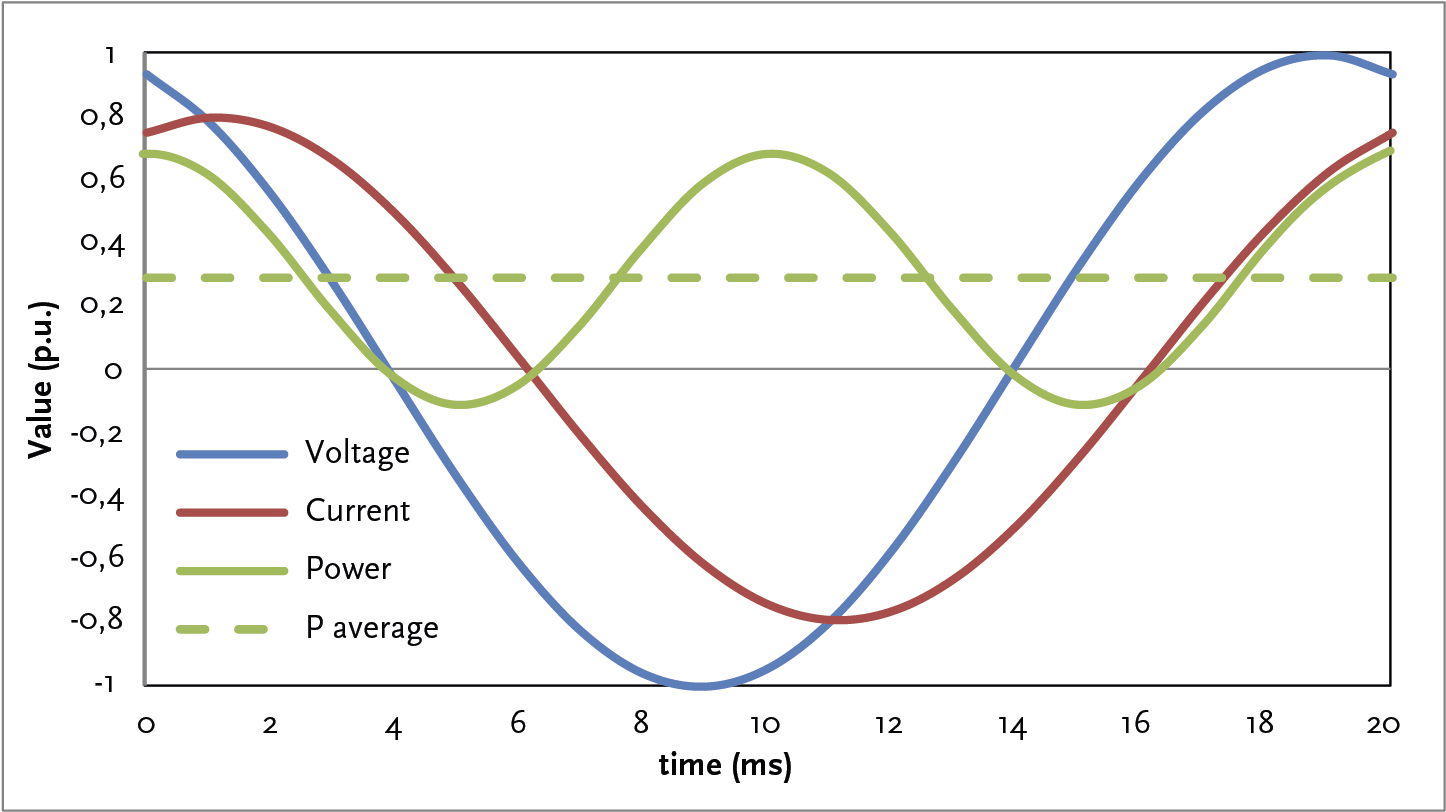
In the case of a purely inductive load, a 90-degree lagging current is generated with φ = 90·(2π/360) rad and figure 7.6 is created. In this figure, it is noticeable that the instantaneous power is as often positive as it is negative-sequence. The average power, with which work is performed, has in that case become equal to zero because cos(φ) is now equal to 0. This means that no active power is being transmitted in this case. That is correct, because this is a characteristic of an ideal inductor.
The average power Paverage, with which work is performed, is equal to the known active power P, expressed in Watts (W).
 |
[ |
7.10 |
] |
The product of the effective value of voltage and current is called the apparent power, denoted in S, expressed in Volt-Amperes (VA). This is a very important value because all installations are designed based on the apparent power. This design parameter is listed on the nameplate of, among other things, transformers.
 |
[ |
7.11 |
] |
This allows the reactive power Q, the power component with which no work can be performed, to be calculated. It is expressed in VAR.
 |
[ |
7.12 |
] |
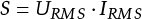
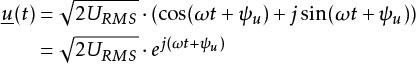
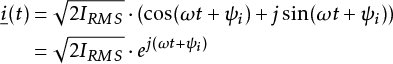
In addition to a varying cosine function, the voltage can also be represented by a rotating vector in the complex plane. The vector rotates at the same speed as the rotor of a generator, which is composed of two magnetic poles. The speed is expressed in the angular frequency ω and can be found as such in equations 7.1 and 7.2. Figure 7.7 illustrates this.
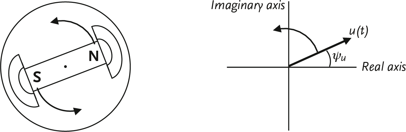
The rotating pointer is described by extending the cosine time function of equation 7.1 with an imaginary part, resulting in the function of the complex instantaneous value. This extended equation describes the position of the arrowhead of the pointer in figure 7.7 in the complex plane as a function of time. The function can be described with cosine and sine terms, but also with a complex exponential.
 |
[ |
7.13 |
] |
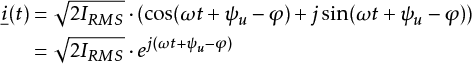
The current is described in the complex plane with the following equation:
 |
[ |
7.14 |
] |
By using equation 7.4, the complex current function from equation 7.14 can also be written as follows:
 |
[ |
7.15 |
] |
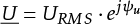
The extended complex equations for voltage (7.13) and current (7.15) form the basis for complex calculations involving currents, voltages, and power. In electrical power engineering, phasors in the complex plane are frequently used. In these calculations, the effective values are always used, and the time dependency is omitted. The relationship between the effective value and the peak value is a factor √2. The time dependency is represented in the complex exponential notation by the term ejωt. If equation 7.13 is divided by √2 and by ejωt, this transforms into the time-independent phasor:
 |
[ |
7.16 |
] |
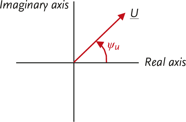
This phasor is a vector in the complex plane, whose length is equal to the effective value URMS of the voltage and the angle at t=0 with respect to the real axis is equal to the voltage phase angle ψu.
This also applies to the current. Similarly, if equation 7.15 is divided by √2 and by ejωt, this converts to the phasor notation for the current:
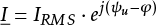 |
[ |
7.17 |
] |
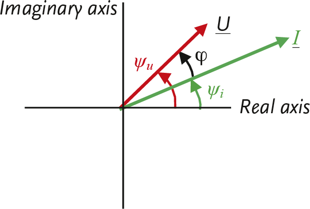
Figure 7.9 illustrates this for the phasors of voltage and lagging (inductive) current. It also shows the relationship between the phase angles of voltage (ψu) and current (ψi) and the phase difference (φ) visible.
The complex power is defined by the phasor S, whose magnitude S equals the apparent power. The real part corresponds to the active power P, and the imaginary part corresponds to the reactive power Q.
 |
[ |
7.18 |
] |
By using equations 7.10 for P and equation 7.12 for Q equation 7.18 becomes S in the following equation, where the cosine and sine terms can also be described with a complex exponential.
 |
[ |
7.19 |
] |
The angle of the power phasor S is therefore entirely determined by the angle φ between the voltage and current phasors U and I. Further elaboration of equation 7.19, by URMS to multiply by ejψu and by IRMS to multiply by e–jψi, yields:
 |
[ |
7.20 |
] |
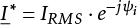
In equation 7.20, it is noticeable that the first term is equal to the voltage phasor U and that the second term, except for the minus sign of the complex exponential, is equal to the current phasor I. For the continuation, the added complex value of the phasor is now considered I defined, for which the imaginary value has an opposite sign:
 |
[ |
7.21 |
] |
As a result, the complex power can be written as follows:
 |
[ |
7.22 |
] |
This last one is the well-known equation by which the complex power is directly determined from the complex voltage and current. This equation is the basis of every power flow calculation.
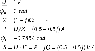
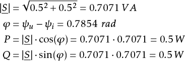
When comparing figure 7.9 with the phasor diagrams given in table 7.2, the relationship between phase angle (leading or lagging) and load type becomes clear. The following calculation example elaborates on this. The starting point is a voltage of 1 V and a load with an inductive impedance of 1+j Ω. Using the motor convention, the following results:
 |
[ |
7.23 |
] |
According to equation 7.23, the active power P is equal to 0.5 W and the reactive power Q is equal to 0.5 var. To verify the correctness of the sign conventions for the powers and the phase angles, the powers can also be derived from the apparent power and the phase difference between the voltage and the current:
 |
[ |
7.24 |
] |
In which |S| is the modulus (magnitude) of complex apparent power S.
Most alternating current systems are designed as three-phase systems, where the three phases each form an angle of 120 degrees with each other. In radians, the mutual angle is then equal to 2/3 π. Figure 7.10 shows how three pairs of coils, each positioned 120 degrees relative to each other on the stator of a generator, generate the voltages. In the example, the coils are connected in a star configuration. Due to the counterclockwise rotation of the rotor, the phase sequence is: a, b, c.
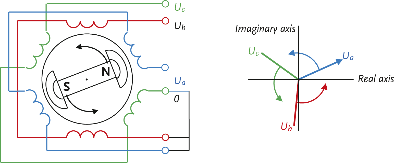
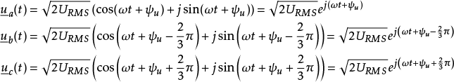
The complex instantaneous voltage of a balanced three-phase voltage source can, by analogy with equation 7.13 in the previous paragraph, be described with the following three time functions for phases a, b, and c. Here, the three voltage phasors are each shifted by 120 degrees relative to each other. In radians, that is –2/3 π and –4/3 π. The value of –4/3 π corresponds to +2/3 π. In the functions for the three voltages, the ψu for the three phases respectively the values 0, –2/3 π and +2/3 π added.
 |
[ |
7.25 |
] |
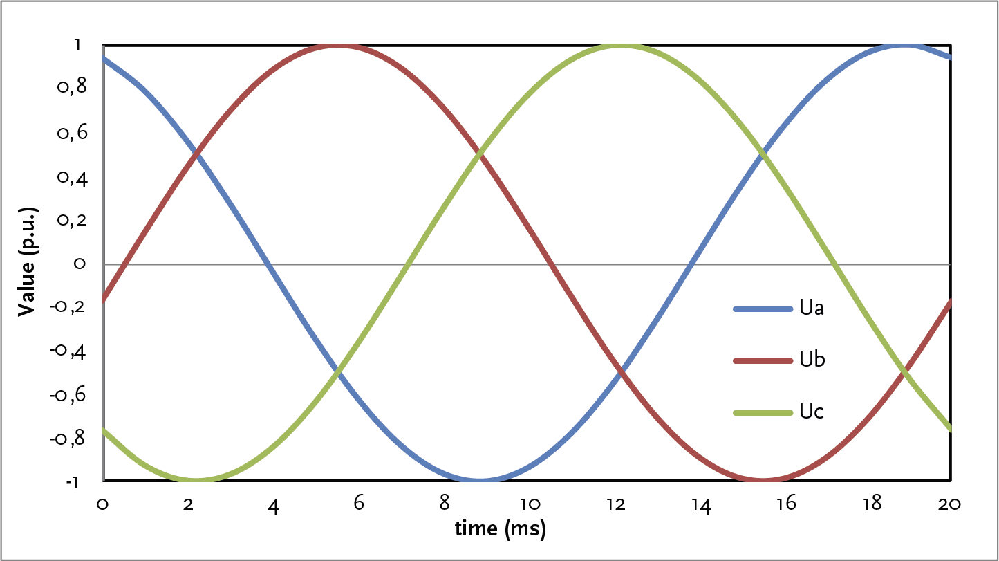
In the above equations, yu is the angle of the voltage of phase a at t = 0. Figure 7.11 illustrates this, showing that the phase sequence is: a-b-c. In the image, ψu is taken as zero.
Calculations for three-phase systems require simultaneous consideration of all three phases of the entire system. The calculations become much simpler if it is assumed that the voltages in the system are perfectly three-phase symmetrical, or balanced. In that case, a three-phase system is modeled as if only one phase is present. The voltages in the other phases can then be easily derived because it is known that they differ by plus or minus 120 degrees from the calculated phase. Henceforth, it is assumed that the power sources installed in the network provide a balanced voltage. The cables and transformers are modeled as three-phase symmetrical components.
However, there are always causes of imbalance, such as an asymmetrical load or an asymmetrical fault in the network. To avoid reverting to calculations with all phases simultaneously, these types of asymmetrical situations are calculated in most methods using the symmetrical components method. This method was described by Fortescue in 1918. The international standard IEC 60909 for short-circuit calculations also uses this method.
An important premise of the method is that the network is symmetrical. The power supplies are distributed over the three phases, and the connections are three-phase symmetrical. The symmetrical components method transforms a three-phase AC network into three independent single-phase systems, called: respectively: positive-sequence, negative-sequence, and zero-sequence. The Dutch terms for these three systems are respectively: normaal netwerk, invers netwerk, and homopolair netwerk. The specific imbalance at a fault location determines how the three independent single-phase systems (component networks) are interconnected. A significant advantage of this method is that networks and faults in networks can be easily calculated using this method. The method allows for calculations to be performed manually.
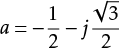
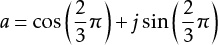
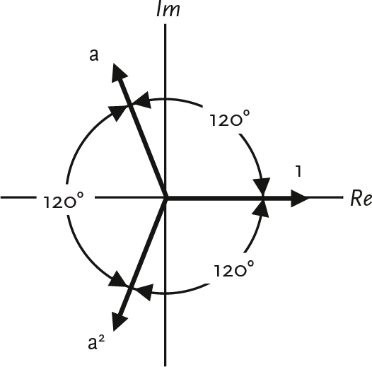
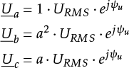
The basis for the symmetrical components method is formed by three vectors in the complex plane, which are shifted 120 degrees from each other and have a length of 1. The method introduces a complex phasor a, with a length of 1 and an angle of 120 degrees relative to the real axis. An angle of 120 degrees is equal to 2/3 π radians. This phasor can be described in various ways:
|
[ |
7.26 |
] |
Multiplying a phasor by a produces a new phasor that is rotated 120 degrees, or 2/3 π, further. Multiplying phasor a by itself yields phasor a², which has an angle of 240 degrees, or 4/3 π, relative to the real axis-equivalent to –120 degrees, or –2/3 π. Figure 7.12 illustrates this for the vectors 1, a and a2.
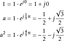
The three phasors are described as complex exponentials or in polar form as follows:
 |
[ |
7.27 |
] |
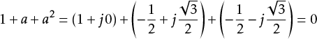
The vector sum of these three phasors is equal to zero. This means that:
 |
[ |
7.28 |
] |
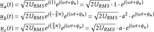
Using these vectors, the equations from equation 7.25 for the instantaneous values of the voltage of a balanced system can also be written as follows:
 |
[ |
7.29 |
] |
It is noted that e-j 2/3 π is equal to ej 4/3 π. From equation 7.29, it can be concluded that a balanced system of voltage vectors can be described with one counterclockwise rotating vector, multiplied by three vectors that are each shifted by 120 degrees relative to each other.
In the complex phasor notation, the system of equations from 7.29 for a three-phase symmetrical voltage system proceeds in the same way as equation 7.16, by dividing by √2 and by ejωt, resulting in:
 |
[ |
7.30 |
] |
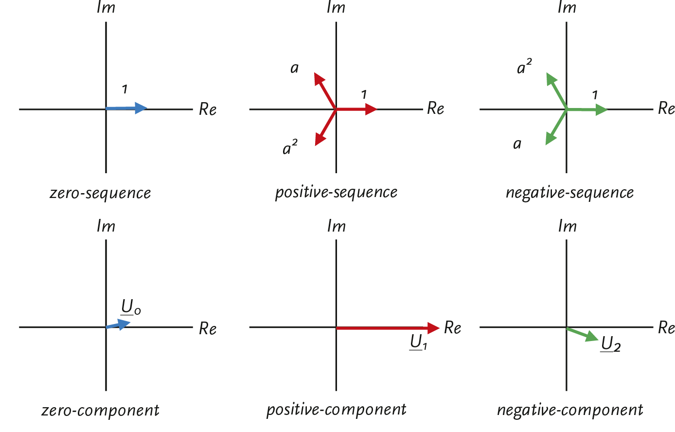
Fortescue’s idea was to represent any arbitrary unbalanced system of vectors using three independent, balanced, counterclockwise rotating vectors: the positive-sequence, negative-sequence, and zero-sequence. In the zero-sequence, the three phasors are equal to each other and are aligned in the same direction. In the positive-sequence, the three phasors are equal to each other and form an angle of 120 degrees relative to each other. In the positive-sequence, the phasors sequence is a-b-c.
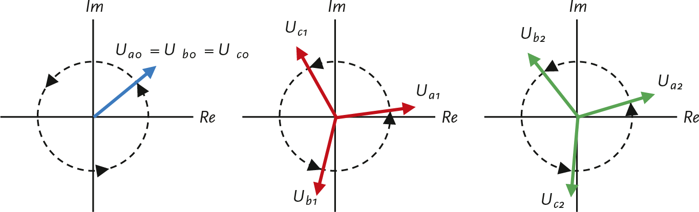
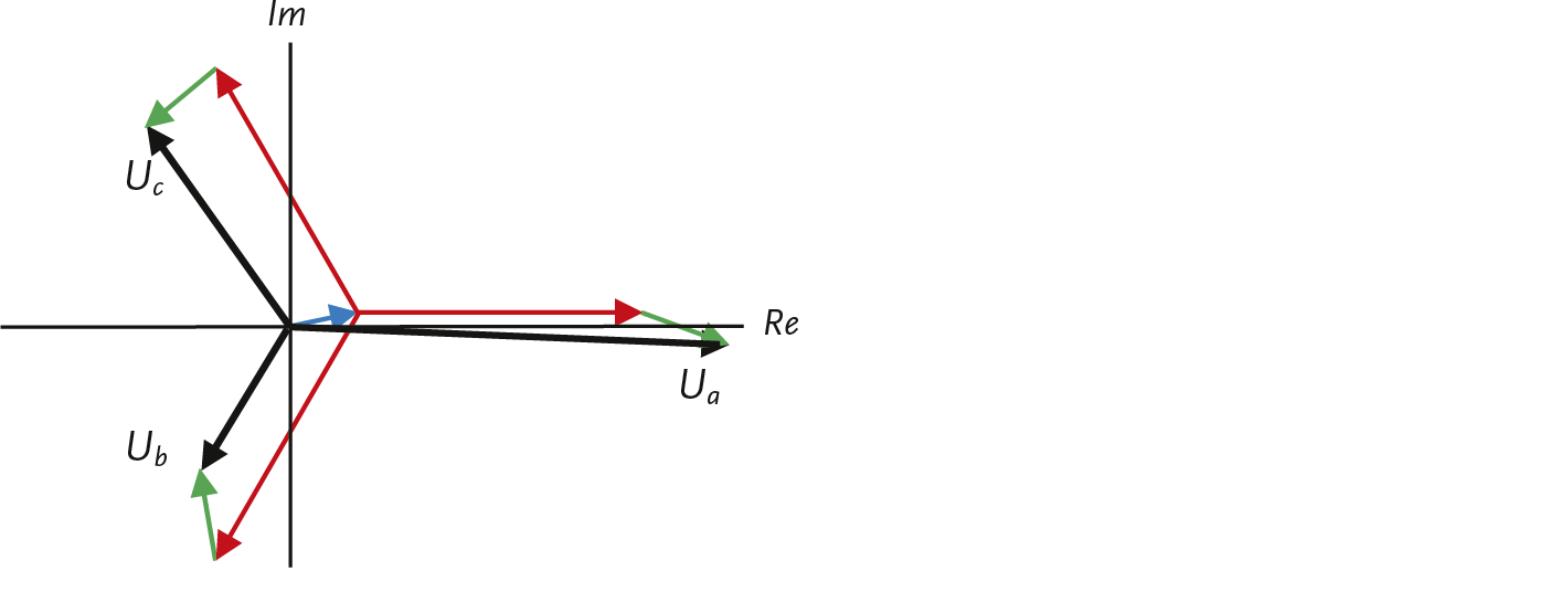
In the negative-sequence system, the three phasors are also equal to each other and form an angle of 120 degrees relative to each other, but the phasor sequence is a-c-b. Each component system has its own specific angular displacement relative to the real axis. These three component systems are depicted above. With the three phasor systems from Figure 7.13, all (asymmetrical) three-phase systems can be constructed. This is illustrated with an example. The following example shows the construction of an arbitrary asymmetrical voltage system.
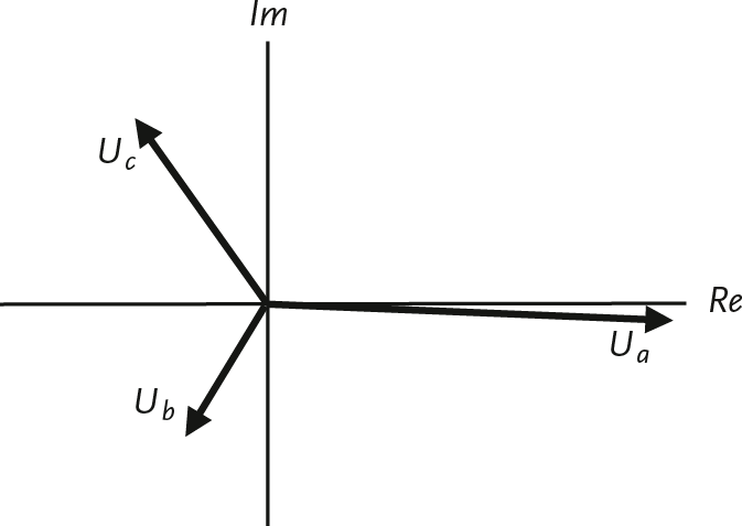
Below, it will be demonstrated using a graphical decomposition that this system can be constructed using:
The asymmetrical system is constructed by adding the vectors for each phase. Thus, for the three phases, the following applies:
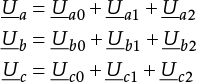 |
[ |
7.31 |
] |
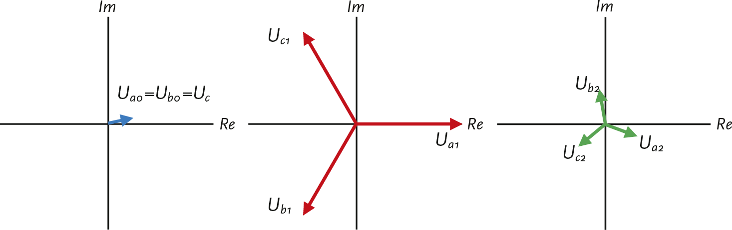
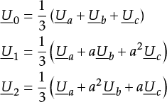
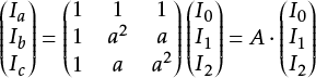
The component voltages of figure 7.15 can be decomposed into three normalized component systems, which are constructed with the phasors 1, a and a2, and three corresponding complex vectors. Figure 7.17 shows the decomposition of the three component systems from figure 7.15.
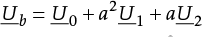
For the system in figure 7.15, all phasors can be described using the three normalized component systems and their complex multiplication factors. In equations 7.32, the multiplication factors are U0, U1 and U2 the complex voltage vectors that determine the effective value and phase angle for each component system. For example, for phase b:
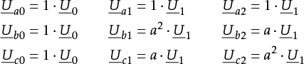 |
[ |
7.32 |
] |
Analogous to equation 7.31, the construction of any three-phase system from the normalized symmetrical components can be described as the sum of the three component voltages:
 |
[ |
7.33 |
] |
This can be converted into a matrix equation. The system of equations 7.33 then transforms into equation 7.34, where matrix A is called the transformation matrix.
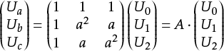 |
[ |
7.34 |
] |
From the example in figure 7.14, the complex values of the three components are:
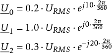 |
[ |
7.35 |
] |
By substituting these values into equations 7.33, the phase values of the asymmetrical voltage system are calculated:
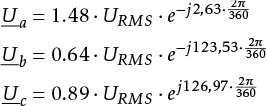 |
[ |
7.36 |
] |
The physical analogy can best be demonstrated with figure 7.18, where an asymmetrical voltage source is described with a series connection of the three component voltage sources. However, it is a fictitious decomposition, as the zero-sequence, negative-sequence, and positive-sequence voltage sources do not actually exist.
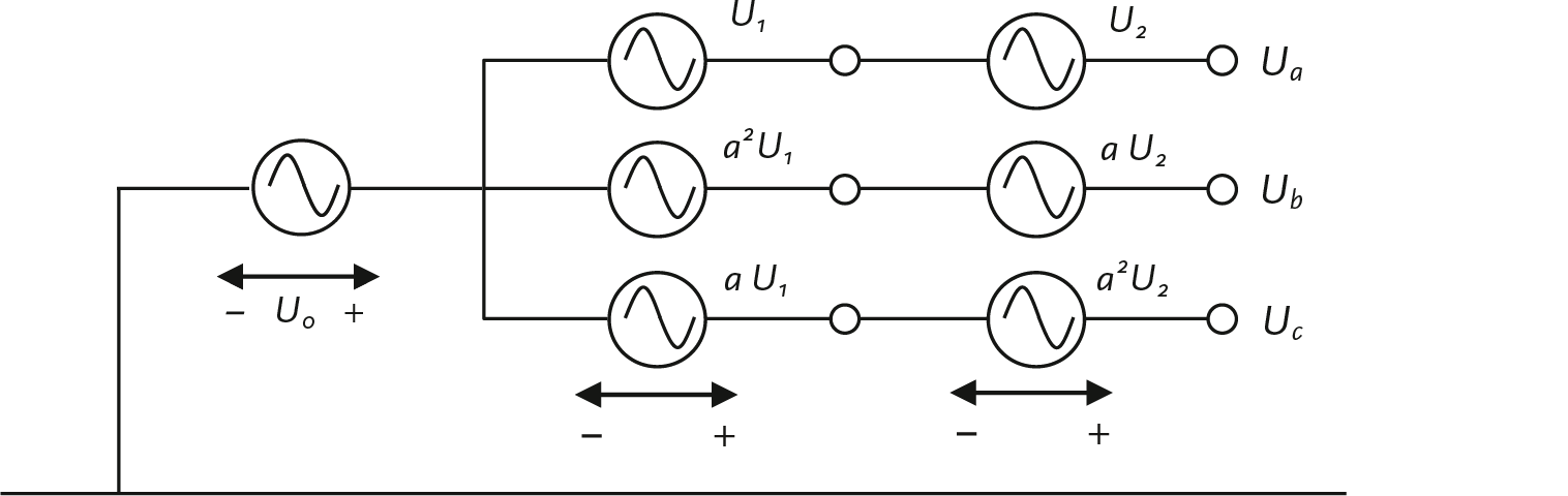
In the ideally balanced case, U0 = 0 and U2 = 0 so that we only have to deal with U1. In practice, however U0≠ 0 and U2≠ 0. This is caused by the imbalance in the three-phase system.
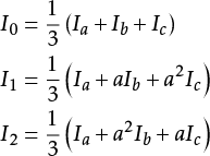
It is therefore possible to measure the physical voltages Ua, Ub and Uc in a three-phase system using the component voltages U0, U1 and U2 Conversely, it is also possible to calculate the component voltages from the physical voltages. By inverting the system of equations from 7.33, the following equations for the decomposition from the physical quantities are obtained.
 |
[ |
7.37 |
] |
This can also be written as a matrix equation. Here, the matrix A-1 is the inverse transformation matrix. This allows the quantities of the component system to be derived from the quantities of the physical system, so that the component stresses are calculated in matrix notation as follows:
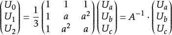 |
[ |
7.38 |
] |
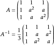
In summary, the following applies to the transformation matrix and the inverse transformation matrix:
 |
[ |
7.39 |
] |
The state in the network is described not only by voltages but also by currents. For the current vectors Iabc and I012 the transformations described above can be performed in the same way. In matrix notation, it looks like this:
 |
[ |
7.40 |
] |
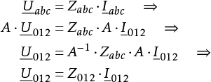
It can be demonstrated that impedances of three-phase systems can also be described using the symmetrical components method. By applying Ohm’s law and using the transformation for the current and voltage vectors, the following results:
 |
[ |
7.41 |
] |
Herein are Uabc, Iabc and Zabc respectively the voltage matrix, the current matrix, and the impedance matrix in the abc system and are U012, I012 and Z012 respectively the voltage matrix, the current matrix, and the impedance matrix in the component system. For the relationship between the impedance matrix in the abc system and the component system, the following applies:
 |
[ |
7.42 |
] |
Each cable connection, transformer, load, and generator can also be modeled with positive-sequence, negative-sequence, and zero-sequence impedances. For most calculations, it is sufficient to assume that the systems are three-phase symmetric. In that case, the system simplifies such that only the positive-sequence impedance needs to be considered. Z1 and the zero-sequence impedance Z0 The positive-sequence impedance is equal to the phase impedance. The negative-sequence impedance does not need to be determined separately, as it is equal to the positive-sequence impedance in this case. The zero-sequence impedance differs from the positive-sequence impedance and must be determined separately. The next paragraph describes an asymmetric power system and the zero-sequence impedance.
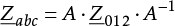
Figure 7.19 is an extension of Figure 7.18, which includes a voltage source with zero-sequence, positive-sequence, and negative-sequence components (U0, U1 and U2) are included. Behind the composite voltage source, an arbitrary three-phase circuit with a return path is included. The three-phase circuit consists of the impedances Za, Zb and Zc, which do not need to be equal to each other. In most three-phase systems, these three impedances are equal to each other, allowing the assumption that the positive-sequence impedance Z1 is equal to the phase impedance, for example Za. The negative-sequence impedance Z2 is then equal to the positive-sequence impedance. There is a return path with a return impedance ZE . The return path can be a fourth conductor, as in low-voltage cables, and it can run through the ground, as in medium-voltage networks.
The component transformation derived from equations 7.40 describes the relationship between the currents in the fictitious component network and the physical system:
| [ |
7.43 |
] |
From this, it appears that the zero-sequence current is equal to one-third of the sum of the three phase currents. In the case of a perfectly balanced three-phase system, the zero-sequence current will be zero. In the case of an unbalanced system, a return current flows, and it can be deduced from figure 7.19 that this is equal to the vector sum of the three phase currents and thus is equal to: IE = Ia+ Ib+ I cc = 3I0.
From this, a method can be derived to measure the zero-sequence impedance. This is done by applying a zero-sequence voltage to the three parallel-connected phases, as shown in figure 7.20. The amplitudes of the positive-sequence and negative-sequence voltage sources (U1 and U2) are, in that case, zero.
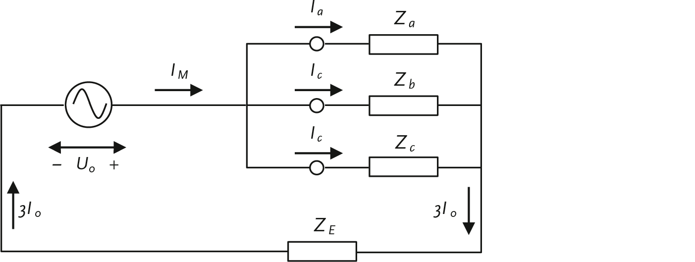
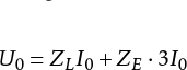
In a balanced three-phase symmetrical network, the following applies to the line impedance to be measured: ZL = Za = Zb = Zc, so the following applies to the currents: Ia = Ib = Ic = I0. Then it can be deduced from the image that for the measurement:
 |
[ |
7.44 |
] |
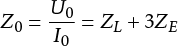
From the above equation, it follows for the zero-sequence impedance:
 |
[ |
7.45 |
] |
During the measurement, three phases are short-circuited, and therefore the parallel connection of three zero-sequence impedances is measured: IM = 3I0. As a result, the zero-sequence impedance from the measurement is determined by multiplying the measured impedance by 3.
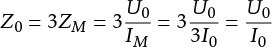 |
[ |
7.46 |
] |
The zero-sequence impedance is thus determined by the entire return circuit, which consists of the neutral conductor (if present), the shielding and armoring of the cable, the ground, conductive pipes, tram and train rails, and all other conductive objects in the return circuit. This makes it so difficult to calculate the value of the zero-sequence impedance. For this reason, it is advisable to measure the zero-sequence impedance of important circuits before they are put into operation.
In many computational tools, normalized quantities are used instead of actual physical quantities. This is done to make it possible to simultaneously calculate low-voltage, medium-voltage, and high-voltage systems, whose quantities differ numerically from each other. Using physical quantities in computer programs could lead to numerical problems. The normalized quantities are expressed in per unit (pu). A second advantage of this method is that manually calculating short-circuit currents across the voltage levels of multiple transformers becomes much simpler.
All quantities are normalized using base quantities. A number of base quantities are chosen, after which the remaining base quantities are derived. Usually, the base quantity for voltage and power is chosen, after which the base quantities for current and impedance are derived. If the base quantity for power is chosen arbitrarily and the base quantity for voltage is taken to be equal to the nominal voltage per voltage level, the following applies to the base quantities:
| Sbase | choice for a 3-phase base power | (MVA) |
| Ubase | coupled voltage per voltage level | (kV) |
| Ibase | base phase current: 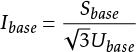 |
(kA) |
| Zbase | base impedance: 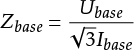 |
(Ω) |
If in the relationship for the base impedance, the numerator and denominator are multiplied by Ubase, it becomes:
| Zbase | base impedance: 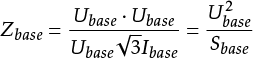 |
(Ω) |
The relationship between power, voltage, current, and impedance is thus determined:
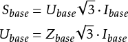 |
[ |
7.47 |
] |
The normalized quantities are then derived from the physical quantities and their base quantities as follows:
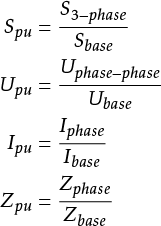 |
[ |
7.48 |
] |
As a result, Ohm’s law applies:
 |
[ |
7.49 |
] |
By dividing both sides of the equal sign by the base voltage, according to the above definition, the same expression in per unit follows:
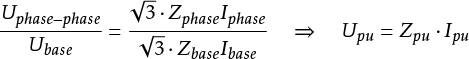 |
[ |
7.50 |
] |
When using the per unit system, the following applies to the per unit values:
Phase to Phase, a subsidiary of Technolution. © 2009-2025