Chapter 12 provides an introduction to the security of supply. It is based on the processes of failure, restoration, and repair.
The translation of ‘Networks for Electricity Distribution’ was created with the help of artificial intelligence and carefully reviewed by subject-matter experts. Even with our combined efforts, a few inaccuracies may still remain. If you notice anything that could be improved, we’d love to hear from you.
In addition to safety, load capacity, and the power quality discussed in the previous chapter, security of supply is one of the quality aspects on which a distribution network is assessed. Availability is determined by planned unavailability and unplanned unavailability (UU). Planned unavailability is caused by maintenance and work on the network. In medium-voltage (MV) networks, maintenance will almost never lead to planned unavailability. Unplanned unavailability is caused by spontaneously occurring failures in components. Depending on the function of a network, a failure may or may not lead to an interruption in the electricity supply. A transmission network is usually designed and protected in such a way that a failure leads to the immediate shutdown of the faulty component, allowing the supply to continue uninterrupted. In the MV distribution network, a cable failure, due to the chosen protection philosophy, will in most cases lead to a shutdown of the faulty section. Only after isolating the short-circuited cable segment can the supply be resumed via an alternative route.
In the past, cost considerations led to the decision that a fault in the distribution network would result in an interruption. Unlike the transmission network, the costs of investments to guarantee uninterrupted supply do not outweigh the costs of the undelivered energy. Only in exceptional situations does the network operator, together with the connected party, opt for a more expensive and reliable connection. Examples include large industrial connections and hospitals. Nevertheless, the likelihood of a supply interruption in the Netherlands is very small. According to the annual fault survey by Netbeheer Nederland, the average availability in 2010 was 99.994%. The average outage duration was 33.7 minutes per year. Interruptions in the medium-voltage network have the largest share in the total average outage duration (Kema, 2011). In 2009, the average outage duration was 26.5 minutes per year. The five-year average is 30.2 minutes per year.
Reliability is described using several characteristic terms. Initially, this can be approached from the perspective of the customer. The reliability of the supply is characterized by:
The annual average outage duration is a measure of the quality of delivery and is equal to the product of the interruption frequency and the average interruption duration:
 |
[ |
12.1 |
] |
The average amount of non-delivered energy (NDE) to a customer or a group of customers is equal to the product of the annual outage duration p, corrected to hours per year) and the average delivered power Pavg in kW.
 |
[ |
12.2 |
] |
Not every fault leads to the failure of a component or an interruption in supply. Due to redundancy, interruptions caused by faults in the HV network occur relatively the least often. In 2010, the percentage of faults that resulted in an interruption was 96.7% for the LV network, 80.9% for the MV network, and 39.8% for the HV network. There are three levels of increasing consequences:
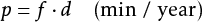
Figure 12.1 provides an overview of the average outage duration (p) in minutes per year per customer from 2000 to 2010 (Kema, 2011). The influence of outages in the LV, MV, and HV networks can be clearly distinguished here. It is evident that the contribution of outages in the LV network remains fairly constant over the years, while the contribution of outages in the MV and HV networks shows considerable variations. The average contribution of outages in the MV network fluctuates between 12 and 23 minutes per year. This is due to the fact that outages occur much less frequently in the MV networks compared to the LV networks, while the consequences of the outages are much greater. The average contribution of outages in the HV network fluctuates even more, between 1 and 11 minutes. For instance, in 2007, there were two major outages in the HV network, causing some circuits of branches that could not be switched over, to be disrupted. The first case involved damage due to ice, and the second case involved a helicopter accident. In 2010, there was a busbar fault due to leakage in a closed SF6-installation, a short circuit in a transformer field, and a defective current transformer were the causes of three interruptions in the high-voltage network, which together led to a significant outage duration.
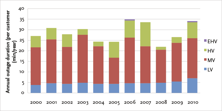
Figure 12.2 provides an overview of the average interruption duration (d) per outage, caused by failures in the LV, MV, HV, and EHV networks, in minutes, for the years 2000 through 2010. It is clear that the average interruption duration due to failures in the LV network is the highest. In most LV networks, there is no switching capability, so the supply is restored by repair or by deploying a temporary back-up generator. Due to the relatively large number of failures, the average interruption duration shows little fluctuation over the years. In 2010, the average interruption duration due to failures in the LV network was 154 minutes.
The average interruption duration due to failures in the MV network also shows little fluctuation over the years. Because the MV network is very extensive, failures occur relatively frequently. The average duration is shorter than for failures in the LV network because in the MV network, the supply is almost always restored by switching. In 2010, the average interruption duration due to failures in the MV network was 89 minutes.
The average interruption duration due to failures in the HV and EHV networks shows significant fluctuations over the years, as it is highly dependent on random incidents. In 2010, the average interruption duration due to failures in the HV network was 63 minutes.
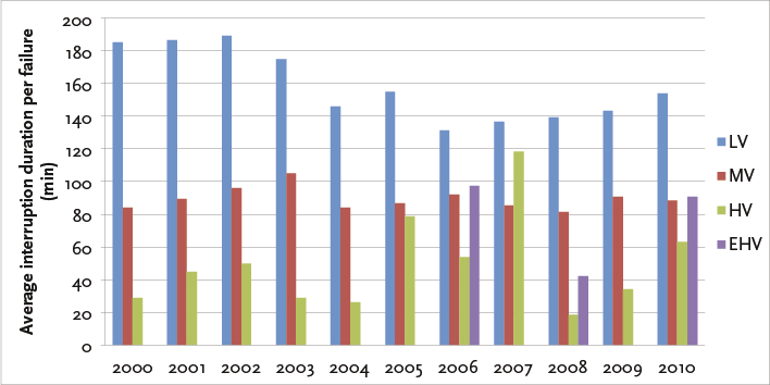
Figure 12.3 shows the average interruption frequency (or interruption expectation, f) of a connected user due to failures in the LV, MV, HV, and EHV networks, in number of interruptions per year. The graph is not included in the report of the annual outage survey but can be easily calculated using the relationship in formula 12.1 from the annual outage duration (Figure 12.1) and the average interruption duration (Figure 12.2). Figure 12.3 shows that the interruption frequency for a connected user due to failures in the LV network is the smallest. In 2010, the interruption frequency due to failures in the LV network was 0.046 times per year, or once every 22 years.
The interruption frequency due to failures in the MV network is, however, much higher than due to failures in the LV network. This is because the MV network that supplies a particular customer is much more extensive than the specific LV network that supplies the same customer. In 2010, the interruption frequency for a customer due to failures in the MV network was 0.21 times per year, or once every 5 years.
The interruption frequency due to failures in the HV network is again smaller than due to failures in the MV network. This is because the HV network is designed in such a way that a single failure is immediately disconnected by the protection system, after which the network continues to function. Only in cases where there is no single failure reserve, or if a double-circuit connection of a feeder goes out of service, will the supply be interrupted. In 2010, the interruption frequency for a customer due to failures in the HV network was 0.12 times per year, or once every 8 years.
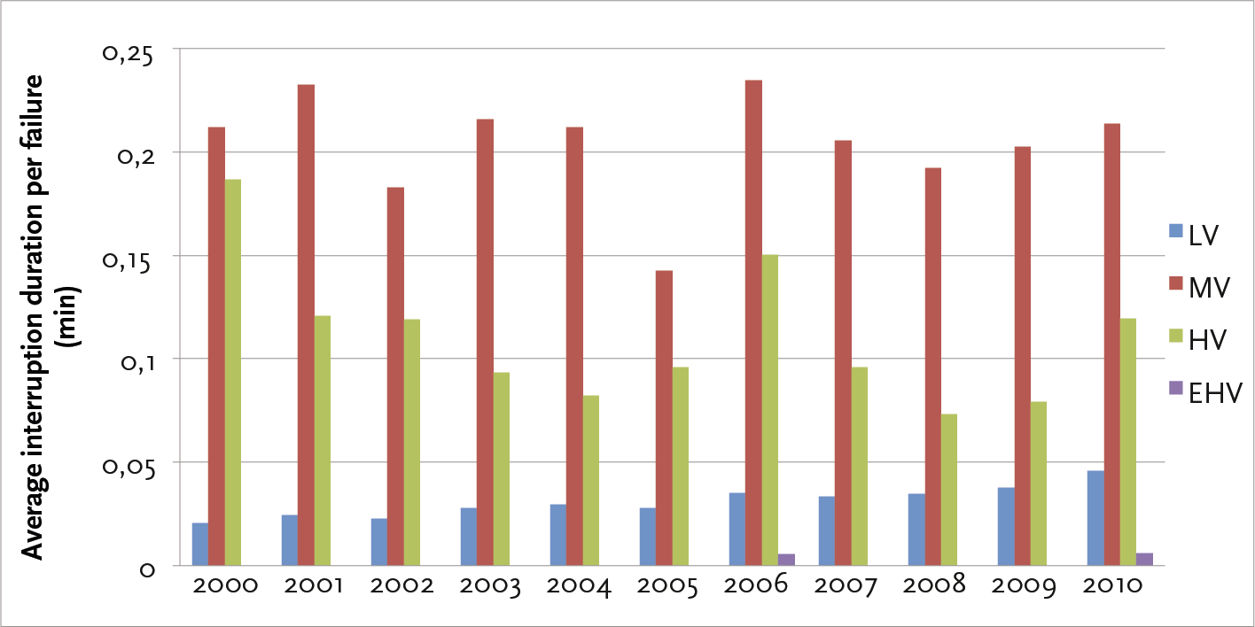
Table 12.1 provides an overview of the average values from the years 2000 to 2010 of the failure data, which are derived from the data in Figure 12.1, Figure 12.2, and Figure 12.3. The table presents the failure data for a customer connected to the LV network due to failures in the LV, MV, and HV networks. It is clear that the average annual outage duration (p) due to failures in the LV network is of the same order of magnitude as that due to failures in the HV network, but that in the HV network relatively frequent short interruptions occur, while in the LV network relatively many long-term failures occur. Due to the size of the MV network, this contributes the most to the annual outage duration. For this reason, it is important to pay a lot of attention to the reliability of the MV network.
Characteristic |
Cause in |
||||
< 1kV LV |
1..35 kV MV |
35..220 kV HV |
Total |
Unit |
|
Interruption expectation (f) |
0.03 |
0.20 |
0.11 |
0.34 |
per year |
Average interruption duration (d) |
158 |
90 |
50 |
83 |
min |
Annual outage duration (p) |
4.8 |
18.3 |
5.5 |
28.6 |
min/year |
In English-speaking countries, terms used to define reliability data are based on the number of affected connections. Although defined slightly differently, the values are equivalent to the outage characteristics used in the Netherlands.
This term is equivalent to the interruption expectation or interruption frequency (f) of the supply. SAIFI is the average number of interruptions that a connected customer can expect and is calculated as follows:
 |
[ |
12.3 |
] |
The number of interruptions for connected customers usually pertains to a year. For North American network operators, the average value is 1.1 interruptions per customer per year (IEEE Standard 1366-1998). In the Dutch grids, according to Table 12.1, this was an average of 0.34 per year for the period 2000-2010.
This term is equal to the annual outage duration (p). SAIDI is the expected outage duration for each connected customer and is calculated as follows:
 |
[ |
12.4 |
] |
SAIDI is measured in minutes and usually pertains to a year. For North American network operators, the average value is 90 minutes per customer per year. In the Dutch grids, according to table 12.1, this was an average of 28.6 minutes per year for the period 2000-2010.
This term is equal to the average interruption duration (d). CAIDI is related to SAIFI and SAIDI in a manner similar to the relationship in formula 12.1:
 |
[ |
12.5 |
] |
CAIDI is the average outage duration that a customer can expect and can also be seen as the average restoration time. For North American network operators, the average value is 82 minutes. In the Netherlands, according to Table 12.1, this was an average of 83 minutes for the period 2000-2010.
This term is equal to the average amount of energy not served (ENS) to a customer or a group of customers. EENS is equal to the product of the annual outage duration and the average delivered power in kW:
 |
[ |
12.6 |
] |
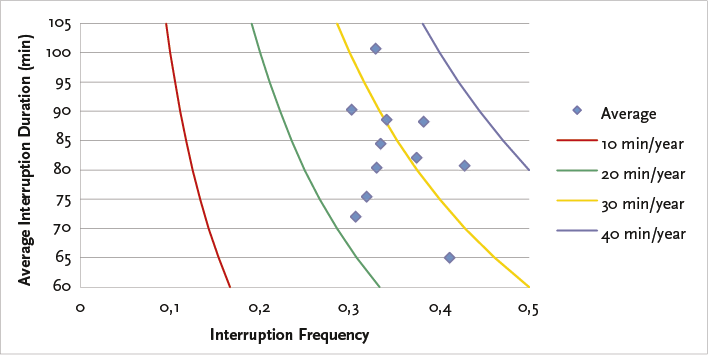
On average, in 2010, a customer experienced 0.38 interruptions. Figure 12.4 provides an overview of the average interruption duration versus the average interruption frequency for the years 2000 through 2010. Each marker represents an annual average. During the period considered, the interruption frequency varied f ) between 0.31 and 0.42, and the interruption duration varied (d) between 65 and 101 minutes. There is no correlation between the frequency and the duration. The curves represent the constant annual outage duration (p) increasing by 10 min/year and based on the product of interruption frequency (f) and interruption duration (d).
Compared to other European countries, the Dutch electricity supply system has a high reliability. In Europe, the annual averages for interruption duration range from 30 to 100 minutes, but also include high values of 200 to 300 minutes. Similarly, the annual averages for interruption frequency in Europe show high values of up to 2 times per year (Kema, 2011).
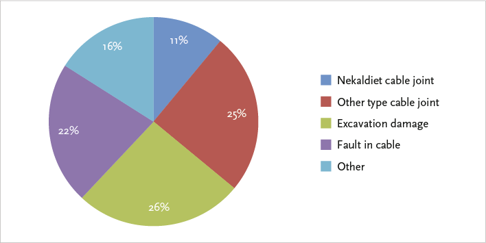
The distribution network is almost entirely laid underground. Records have shown that excavation work is one of the main causes of interruptions. To reduce the number of excavation damages, the Information Exchange Act for Above- and Below-Ground Networks (WIBON) regulates the exchange of information about the location of cables and pipelines. Additionally, interruptions in cable joints are notorious. Figure 12.5 provides an overview of the main causes of interruptions in the medium-voltage network of a network operator (Alliander, 2009). This overview clearly shows that the vast majority of all interruptions are related to cables and their accessories. It can be seen that approximately one-third of the interruptions are caused by joints and one-quarter by excavation damage. About one-fifth of the interruptions are due to a defect in a cable. For instance, the thermal expansion and contraction, caused by a high fluctuating load, is a significant cause of accelerated aging of a PILC cable.
The reliability of medium-voltage (MV) distribution networks is most affected because the N–1 reserve is structural rather than operational, unlike in transmission networks. Every short circuit results in the disconnection of the entire section. Detecting the fault and switching after a failure is done manually, which takes more time than in a transmission network, which is equipped with remotely readable measurements and remote control. Moreover, the consequences of a failure in the MV distribution network are quite significant, as the failure of a section affects a relatively large number of connected users.
Each network operator uses its own reliability criteria. The average interruption duration for the different levels is adjusted based on the costs associated with not delivering energy. In low-voltage (LV) networks, sometimes an absolute duration is used for the average interruption. In other cases, such as at the medium-voltage (MV) level, the criterion is that the amount of undelivered energy, the product of the average restoration time and total affected load, must not exceed a specific value, in MWh. Additionally, in certain situations, a connected user can agree on reliability requirements with the network operator.
Reliability is determined by the combination of two processes: the failure of a component and the restoration of the supply to the disconnected subnet. It is not always the case that the supply is only resumed after the faulty component has been repaired. Therefore, in addition to knowledge about the repair data, insight into the restoration process of the supply is also needed. The failure of a component and the restoration of the supply are two separate processes that are approached independently.
The failure frequency and repair duration of the individual components are defined:
The failure and repair data of components in the grid are listed in the annual outage survey of Netbeheer Nederland (Kema, 2011). This annual report includes the recorded outages of that year. Given the relatively small number of outages, the data can vary significantly from year to year, both in the number of outages and in repair duration. There are also differences in failure frequency and repair time per network operator. For example, a network operator may have used joints of a certain type from a specific manufacturer in the past, which all show the same signs of degradation over time. Differences in repair strategies can also lead to variations in repair times. Tables 12.2, 12.3, and 12.4 provide an overview of the outage data of components in the LV, MV, and HV networks in the Netherlands for the years 2007, 2008, 2009, and 2010. The repair duration is the average recovery time of a component whose failure led to interruptions in supply.
Failure frequency |
Repair duration (h) |
||||||||||
Component |
2007 |
2008 |
2009 |
2010 |
Average |
Unit |
2007 |
2008 |
2009 |
2010 |
Average |
Network cable PILC |
0.0465 |
0.0441 |
0.0440 |
0.0502 |
0.0462 |
/km |
6 |
10 |
10 |
24 |
13 |
Network cable XLPE |
0.0347 |
0.0308 |
0.0288 |
0.0352 |
0.0324 |
/km |
5 |
7 |
9 |
16 |
9 |
Connection cable PILC |
0.0952 |
0.1028 |
0.0975 |
0.0578 |
0.0883 |
/km |
6 |
13 |
27 |
30 |
19 |
Connection cable XLPE |
0.0658 |
0.0689 |
0.0624 |
0.0816 |
0.0697 |
/km |
4 |
8 |
17 |
19 |
12 |
PILC cable joint |
0.0002 |
0.0002 |
0.0003 |
0.0005 |
0.0003 |
/each |
8 |
9 |
15 |
35 |
17 |
XLPE cable joint |
0.0002 |
0.0001 |
0.0002 |
0.0003 |
0.0002 |
/each |
8 |
11 |
14 |
32 |
16 |
PILC end termination |
0.0001 |
0.0001 |
0.0001 |
0.0000 |
0.0001 |
/each |
5 |
4 |
4 |
11 |
6 |
XLPE end termination |
0.0001 |
0.0001 |
0.0001 |
0.0001 |
0.0001 |
/each |
3 |
3 |
9 |
18 |
8 |
Fused load break switch |
0.0016 |
0.0017 |
0.0015 |
0.0014 |
0.0016 |
/each |
2 |
2 |
2 |
3 |
2 |
Low-voltage rack, cabinet |
0.0011 |
0.0012 |
0.0012 |
0.0017 |
0.0013 |
/each |
3 |
8 |
16 |
69 |
24 |
Fuse |
0.0012 |
0.0013 |
0.0014 |
0.0017 |
0.0014 |
/each |
2 |
2 |
4 |
6 |
4 |
Table 12.2 shows that the variation over the years in the failure frequency of low-voltage cables is between 5 and 20%. In particular, PILC cables are more prone to disturbances than XLPE cables. It is also notable that the failure frequency of low-voltage connection cables is twice as high as that of grid cables. The variation in repair duration is especially significant for connection cables. For grid cables, the repair duration is expected to be around 8 to 12 hours. It is anticipated that the repair duration for a joint is approximately the same as for a cable.
MV |
Failure frequency |
Repair duration (h) |
|||||||||
Component |
2007 |
2008 |
2009 |
2010 |
Average |
Unit |
2007 |
2008 |
2009 |
2010 |
Average |
Cable PILC |
0.0114 |
0.0108 |
0.0110 |
0.0128 |
0.0115 |
/km |
87 |
92 |
154 |
120 |
113 |
XLPE cable |
0.0069 |
0.0078 |
0.0101 |
0.0048 |
0.0074 |
/km |
101 |
66 |
93 |
149 |
102 |
PILC cable joint |
0.0026 |
0.0029 |
0.0032 |
0.0037 |
0.0031 |
/each |
96 |
65 |
150 |
126 |
109 |
Oil-filled joint |
0.0004 |
0.0003 |
0.0005 |
0.0004 |
0.0004 |
/each |
213 |
105 |
159 |
150 |
157 |
XLPE joint |
0.0019 |
0.0018 |
0.0010 |
0.0011 |
0.0015 |
/each |
89 |
59 |
105 |
76 |
82 |
PILC end termination |
0.0001 |
0.0000 |
0.0001 |
0.0001 |
0.0001 |
/each |
50 |
38 |
346 |
63 |
124 |
Oil-filled end termination |
0.0001 |
0.0001 |
0.0002 |
0.0002 |
0.0002 |
/each |
77 |
51 |
164 |
163 |
114 |
XLPE end termination |
0.0002 |
0.0001 |
0.0002 |
0.0002 |
0.0002 |
/each |
28 |
25 |
54 |
97 |
51 |
Rail |
0.0002 |
0.0001 |
0.0003 |
0.0004 |
0.0003 |
/each |
126 |
128 |
33 |
125 |
103 |
Transformer MV/LV |
0.0007 |
0.0006 |
0.0008 |
0.0006 |
0.0007 |
/each |
105 |
31 |
59 |
70 |
66 |
Circuit breaker |
0.0019 |
0.0019 |
0.0013 |
0.0009 |
0.0015 |
/each |
22 |
26 |
88 |
64 |
50 |
Load Break Switch |
0.0002 |
0.0002 |
0.0002 |
0.0002 |
0.0002 |
/each |
43 |
60 |
71 |
53 |
57 |
Load separator |
0.0001 |
0.0000 |
0.0001 |
0.0001 |
0.0001 |
/each |
236 |
1 |
13 |
154 |
101 |
Current limiting reactor |
0.0000 |
0.0000 |
0.0005 |
0.0000 |
0.0001 |
/each |
2620 |
2620 |
|||
Table 12.3 shows that the failure frequencies of components in the MV network are lower than those of components in the LV network: the failure frequency of cables is approximately four times lower. Here too, PILC cables are more frequently disturbed than XLPE cables. This is not necessarily due to the age or quality of the cables. PILC cables are typically located in older urban areas, where they can be damaged by excavation work for urban renewal projects.
It is immediately noticeable that the repair duration for medium-voltage (MV) cables is much longer than for low-voltage (LV) cables. Additionally, the variation in repair duration over the years is quite large. In general, repairs in 2009 and 2010 seem to take longer than in the previous two years. The fact that the repair durations for MV cables are longer than for LV cables is because, in the event of failures in MV cables, the supply can usually be restored by switching, making the repair less urgent. For other components, such as rails, transformers, circuit breakers, and current limiting reactors, the repair duration is the time required to replace the defective component. The failure frequency of these components is so low that the repair duration has a fairly large variation, making it difficult to find a realistic value. For instance, there is only one record of current limiting reactor replacement in 2009, where the replacement duration was apparently very long.
HV |
Failure frequency |
Repair duration (h) |
|||||||||
Component |
2007 |
2008 |
2009 |
2010 |
Average |
Unit |
2007 |
2008 |
2009 |
2010 |
Average |
Cable |
0.0047 |
0.0025 |
0.0032 |
0.0037 |
0.0035 |
/km |
145 |
235 |
102 |
397 |
220 |
Overhead line |
0.0060 |
0.0036 |
0.0038 |
0.0057 |
0.0048 |
/km |
433 |
7 |
4 |
210 |
164 |
Joint |
0.0000 |
0.0000 |
0.0001 |
0.0000 |
0.0000 |
/each |
|||||
End termination |
0.0014 |
0.0013 |
0.0007 |
0.0004 |
0.0010 |
/each |
730 |
99 |
89 |
11 |
232 |
Circuit breaker |
0.0012 |
0.0032 |
0.0044 |
0.0016 |
0.0026 |
/each |
48 |
18 |
161 |
3 |
58 |
Load separator |
0.0004 |
0.0002 |
0.0006 |
0.0005 |
0.0004 |
/each |
3 |
4 |
6 |
1652 |
416 |
Rail |
0.0014 |
0.0015 |
0.0042 |
0.0109 |
0.0045 |
/each |
10 |
10 |
|||
Transformer HV/MV |
0.0021 |
0.0197 |
0.0196 |
0.0205 |
0.0155 |
/each |
67 |
38 |
123 |
67 |
74 |
Table 12.4 shows that the failure frequency of components in the HV network is generally lower than that of components in the MV network. In general, the average repair duration is longer than that of components in the MV network. Because the HV network is relatively small compared to the MV and LV networks, there are relatively few failures, resulting in a wide variation in repair duration.
Failure is defined as a component becoming so defective that it is immediately taken out of service. The interruption frequency (f) of a branch is calculated from the sum of the failure frequencies (λ) of all components of the branch, plus the interruption frequency (fsupply) of the upstream network. Figure 12.6 illustrates that a connected user in the LV network deals with the chain of reliability of the LV network, the substation, the MV network, the feeder station, and the HV and EHV networks. If a short circuit occurs in one of the cables of an MV branch, the protection of that branch will activate and disconnect, causing the entire branch, including all connected users, to be out of service.
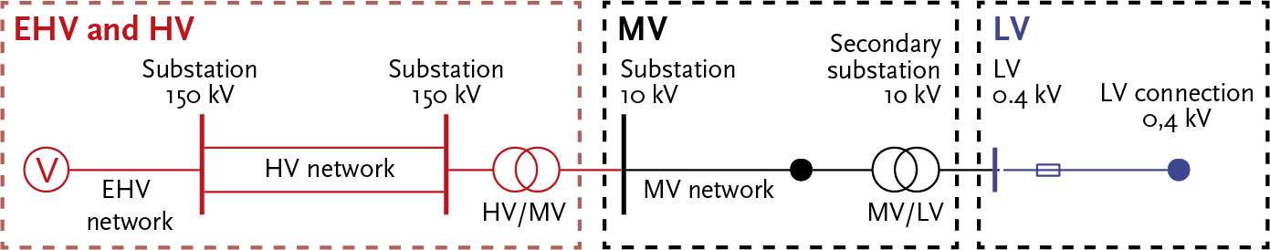
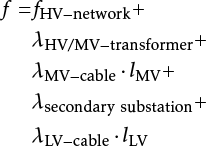
In the following equation, the interruption frequency of a point in the LV network is calculated from the sum of the interruption frequency of the HV busbar of the HV/MV substation and the failure frequencies of the components of the substation up to the LV network. The interruption frequency of the HV network is not calculated but is taken from the fault registration data in Table 12.1, because the reliability calculation of the N-1 secure transmission network requires a more extensive calculation than the method presented in this chapter for distribution networks.
 |
[ |
12.7 |
] |
with:
| f | failure frequency |
| λHV/MV transformer | failure frequency of the power transformer (per year) |
| lMV | length of MV cable (km) |
| λMV cable | failure frequency of MV cable (per year and per km) |
| lLV | length of LV cable (km) |
| λLV cable | voltage phase angle (rad) failure frequency of LV cable (per year and per km) |
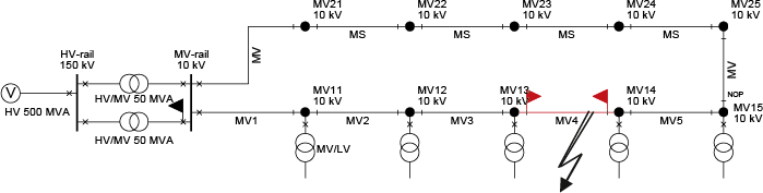
The failure process is explained using the example network in figure 12.7. In this network, the reliability of the EHV and HV network, and thus the reliability of the supply at the HV node of the substation, is modeled in the reliability of the network supply.
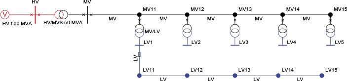
All MV cables in this example are of equal length: 1000 m. Similarly, all LV cables behind substation MV11 are of equal length: 100 m. The failure frequency of a cable is equal to the product of its length and its failure frequency per unit length. The failure frequencies are derived from Table 12.1, Table 12.2, Table 12.3, and Table 12.4. The failure frequency of an MV cable is set at 0.01 km/year and that of an LV cable at 0.03 km/year. The failure frequencies of busbars and nodes are neglected in this example. The failure parameters of the components of the network in Figure 12.7 for use in a reliability calculation are then:
Component |
Failure frequency λ (per year) |
Network supply |
0.11 |
HV/MV transformer |
0.014 |
MV cable (1 km x lMV cable) |
0.01 |
MV/LV transformer |
0.001 |
LV cable (0.1 km x lLV cable) |
0.003 |
A short circuit only affects the part of the network that is jointly protected. This means that in the event of a short circuit in the substation, the supply to the entire underlying medium-voltage (MV) network is interrupted. All cables and substations in the MV branch are jointly protected. In the event of a short circuit in a cable of the MV branch, the supply to that branch and all connected substations is interrupted. All cables in the low-voltage (LV) branch are also jointly protected. In the event of a short circuit in an LV cable, only the supply to all connections on that LV branch is interrupted. This, of course, assumes that the protection is selectively set and functioning properly. By applying formula 12.7, the failure frequency for all network parts can be calculated. Each ‘jump’ in the calculated failure frequency in table 12.6 is caused by a protection device.
Failing component |
Network supply station |
Substation MV11 |
LV node |
||
HV rail |
MV rail |
MV rail |
LV rail |
|
|
Network supply |
0.110 |
0.110 |
0.110 |
0.110 |
0.110 |
HV/MV transformer |
0.014 |
0.014 |
0.014 |
0.014 |
|
5 MV cables |
0.050 |
0.050 |
0.050 |
||
HV/LV transformer |
0.001 |
0.001 |
|||
5 LV cables |
0.015 |
||||
Total |
0.110 |
0.124 |
0.174 |
0.175 |
0.190 |
The failure frequencies (λ) of components are often assumed to be constant. In practice, the failure frequency is not constant but depends, among other things, on the age of the component, the degree of (over)loading in the past, and the maintenance performed. Protections can also fail, in the sense that they may trip incorrectly or fail to trip when they should (protection refusal). In the case of a refusing protection, the backup protection will need to trip, resulting in less selective disconnection.
In addition to the repair duration, the restoration time is important for determining the unavailability. The restoration time is the duration between the moment of the fault and the restoration of supply. In most cases, nothing is repaired yet, and the supply is restored through switching actions after the faulty component has been isolated. The restoration time consists of several steps, each with its own duration:
After a fault has occurred, causing a part of the network to be shut down, it takes a while before the fault is known at the operations center. With an automatic notification, this happens almost immediately. In other cases, the fault only becomes known after customers have reported it by phone.
After the fault is detected, a repair crew is dispatched to the affected area. The time this takes depends on many factors, such as the time of day and traffic conditions. Experience statistics of the relevant network operator play a significant role in this.
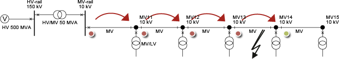
When the troubleshooting team arrives on site, the step for locating the fault site begins. If remotely readable fault indicators are used or a fault location system is employed, the fault site can be found relatively quickly. If that is not the case, the fault site must be located by inspecting the short-circuit indicators station by station. If only one troubleshooting team is working, they can choose between the sequential and binary search methods. In the sequential method, the troubleshooting team checks the status of the short-circuit indicators of all network stations in the affected branch from the substation towards the network opening (Figure 12.8). If the fault is close to the substation, that is advantageous. However, if the fault is at the end of the branch, the search will take a lot of time.
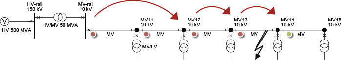
In the binary search method, half of the search area is eliminated each time using a halving method (Figure 12.9). If a short-circuit indicator has detected a continuous short-circuit current, the search continues in the direction of the network opening. If this is not the case, the search moves back toward the substation. Particularly in long branches, the binary search method has an advantage over the sequential search method. This depends on the distances and travel times. In practice, the search method used will be a combination of both methods, where network stations with many branches are visited first, if possible
If the short circuit is located, it is isolated by opening the disconnectors on both sides. In most cases, the short circuit is found in a cable segment or a joint. The short circuit is often caused by excavation work or a spontaneous fault in a cable or joint. If the short circuit is located in a network station, the cables on both sides are disconnected, and the network station can no longer be powered.
In most cable trace faults, the supply is restored by closing the circuit breakers opened by the protection system and by closing one or more disconnectors that are normally open. After the fault location is isolated, the section is split into two parts. The supply to the first part of the section can be easily restored by closing the switch in the substation that was opened by the protection system. The restoration of the supply to the second part of the section can occur in three ways:
Figure 12.10 shows a ring-shaped medium-voltage (MV) network with a network opening at substation ‘MV15’. If the cable between substations ‘MV13’ and ‘MV14’ is short-circuited, the entire section is shut down.
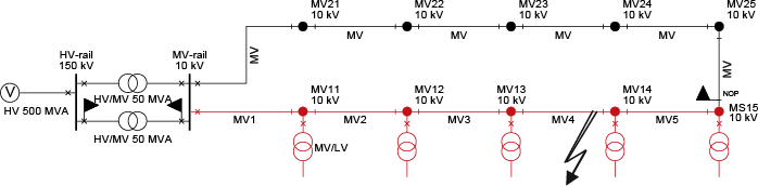
Figure 12.11 shows that the fault was located between substations ‘MV13’ and ‘MV14’, after which the disconnectors on both sides were opened. The supply was restored by, on one hand, switching on the circuit breaker in the substation and, on the other hand, closing the normally open disconnector at substation ‘MV15’.
It depends on the capacity of the network section to be switched whether all substations can be re-energized by closing normally open disconnectors. If the maximum current load of the alternative circuit is insufficient, the supply to the affected substations will, if possible, be distributed over two or more alternative circuits.
In the medium-voltage network, there are branches that cannot be fed from another side by closing normally open disconnectors. In such cases, the supply can only be restored by setting up an emergency power supply. This consists of one or more generators that can be connected to the substations. The repair will be carried out as quickly as possible.
If the short circuit is located in a substation, the supply to the downstream low-voltage (LV) network usually cannot be restored through a switching action. Chapter 2 explains that LV networks are often designed with a radial structure, which lacks a fault reserve. In such cases, the supply can only be restored using an emergency power supply.
If the supply cannot be restored through switching actions or by using an emergency power supply, the outage duration is determined by the repair duration. According to Table 12.2, repairing an LV cable takes approximately 10 hours. According to Table 12.3, repairing an MV cable takes an average of about 100 hours. This repair duration is based on non-urgent repair of a cable in an MV distribution network where the supply has been restored by switching. If the supply cannot be restored by switching, the repair becomes urgent and the cable will be repaired in a shorter time.
The expected repair duration depends on the size of the network and can be calculated from the sum of the time durations involved in all individual repair actions. Table 12.7 provides an overview. The time durations vary from company to company and also depend on the level of automation in each distribution network, the ability to remotely read the short-circuit indicators, and the presence of a fault location system.
Tdetection |
Duration for detecting a short circuit |
Tfault team |
Duration for deploying the fault team |
Tlocalisation |
Duration for locating the fault site |
Tisolation |
Duration for isolating the fault site |
Tswitching on |
Duration for switching on the circuit breaker that was tripped by the protection system |
Tswitching over |
Duration for closing normally open disconnectors |
Temergency power |
Duration for deploying an emergency power supply |
Trepair |
Duration for repairing the faulty component |
It depends on the structure of the network whether the supply can be restored by switching and rerouting or if an emergency power supply needs to be deployed or if it is necessary to wait for repairs. Depending on the method of restoration, the recovery time is determined using the formulas below. Formula 12.8 calculates the recovery for the network section between the substation and the fault location:
 |
[ |
12.8 |
] |
Formula 12.9 calculates the recovery for the network section between the fault location and a network opening:
 |
[ |
12.9 |
] |
Formula 12.10 calculates the recovery for a network section using an emergency power supply:
 |
[ |
12.10 |
] |
Formula 12.11 calculates the recovery for a network section where repair must be awaited:
 |
[ |
12.11 |
] |
For the short circuit in the cable segment between the nodes ‘MV13’ and ‘MV14’, as shown in figure 12.11, the recovery duration of the medium-voltage nodes is explained below. In table 12.8, the time durations of the individual recovery actions are assumed arbitrarily.
Tdetection |
2 minutes |
Tfault team |
30 minutes |
Tlocalisation |
10 minutes per station |
Tisolation |
10 minutes |
Tswitching on |
15 minutes |
Tswitching over |
15 minutes |
Temergency power |
120 minutes |
Trepair |
given per component |
The repair time for a fault in the high-voltage network is taken from table 12.1, which shows the average interruption duration (d) for faults in the high-voltage network is 50 minutes. The repair time for a fault in the high-voltage/medium-voltage supply transformer is determined by the time required to switch to the backup transformer. For this duration, an arbitrary 52 minutes has been assumed. For a fault in one of the cable segments, the repair time by switching on the disconnected circuit breaker in the substation according to formula 12.8 and table 12.8 is equal to: Trepair = 2 + 30 + (5 x 10) + 10 + 15 = 107 minutes. The repair time by switching on the normally open disconnector in substation ‘MV15’ according to formula 12.9 and table 12.8 is equal to: Trepair = 2 + 30 + (5 x 10) + 10 + 15 + 15 = 122 minutes. With this, table 12.9 for the MV nodes of the disturbed section can be compiled.
Failing component |
Restoration time (min) |
|||||
MS rail |
MV11 |
MV12 |
MV13 |
MV14 |
MV15 |
|
Network supply |
50 |
50 |
50 |
50 |
50 |
50 |
HV/MV transformer |
52 |
52 |
52 |
52 |
52 |
52 |
MV cable: MV rail-MV11 |
0 |
122 |
122 |
122 |
122 |
122 |
MV cable: MV11-MV12 |
0 |
107 |
122 |
122 |
122 |
122 |
MV cable: MV12-Mv13 |
0 |
107 |
107 |
122 |
122 |
122 |
MV cable: MV13-MV14 |
0 |
107 |
107 |
107 |
122 |
122 |
MV cable: MV14-MV15 |
0 |
107 |
107 |
107 |
107 |
122 |
By using formula 12.1, table 12.10 for the annual outage duration can be compiled. Here, the calculated repair durations from table 12.9 are multiplied by the outage frequency of the respective failing component. Thus, the annual outage duration for node MV13 for a short circuit in the MV cable between nodes ‘MV12’ and ‘MV13’ is given by:
p = 0.01 x 122 = 1.22 min/year
and for a short circuit in the MV cable between nodes ‘MV13’ and ‘MV14’ given by:
p = 0.01 x 107 = 1.07 min/year.
Failing component |
Annual outage duration (min/year) |
|||||
MV branch |
MV11 |
MV12 |
MV13 |
MV14 |
MV15 |
|
Network supply |
5.50 |
5.50 |
5.50 |
5.50 |
5.50 |
5.50 |
HV/MV transformer |
0.73 |
0.73 |
0.73 |
0.73 |
0.73 |
0.73 |
MV cable: MV rail-MV11 |
0 |
1.22 |
1.22 |
1.22 |
1.22 |
1.22 |
MV cable: MV11-MV12 |
0 |
1.07 |
1.22 |
1.22 |
1.22 |
1.22 |
MV cable: MV12-MV13 |
0 |
1.07 |
1.07 |
1.22 |
1.22 |
1.22 |
MV cable: MV13-MV14 |
0 |
1.07 |
1.07 |
1.07 |
1.22 |
1.22 |
MV cable: MV14-MV15 |
0 |
1.07 |
1.07 |
1.07 |
1.07 |
1.22 |
Total |
6.23 |
11.73 |
11.88 |
12.03 |
12.18 |
12.33 |
The individual contributions to the annual outage duration, as listed in table 12.10, can be summed per node. Thus, the total annual outage duration of substation ‘MV13’ due to all failures in this example is equal to 12.03 minutes (12 minutes and 2 seconds).
Using the calculated failure frequencies from Table 12.6, the average interruption duration for each substation can be calculated using Formula 12.1. All calculated reliability indices for this example are summarized in Table 12.11.
|
MV feeder |
MV11 |
MV12 |
MV13 |
MV14 |
MV15 |
|
Failure frequency (f) |
0.124 |
0.174 |
0.174 |
0.174 |
0.174 |
0.174 |
per year |
Annual outage duration (p) |
6.23 |
11.73 |
11.88 |
12.03 |
12.18 |
12.33 |
min/year |
Average interruption duration (d) |
50 |
67 |
68 |
69 |
70 |
71 |
min |
The economic importance of good reliability is difficult to determine unequivocally. While it is relatively simple to calculate the costs of non-delivered energy (NDE) based on the expected annual outage duration and a price per kWh of unserved energy, the consequences for all connected users are very diverse. For instance, it is assumed that most household users can easily resume their activities after a short interruption. It becomes more challenging when users depend on an uninterrupted supply for data processing. The costs of data loss and restoration efforts can be significant. In production facilities, the consequences of an interruption also vary widely. Some computer-controlled processes come to a complete halt after a very brief interruption. In other processes, such as in the chemical industry, an interruption can lead to the discharge of chemical substances causing environmental damage, and pipelines can become clogged due to the stoppage.
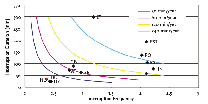
In the Netherlands, an indepent regulator (ACM) monitors reliability using a bonus/malus system. Within Netbeheer Nederland, it has been agreed that each network operator will accurately record reliability according to a mutually agreed system. One of the key parameters published is the average annual interruption duration. This important societal parameter is compared to the national average (Figure 12.1), with the aim of keeping their own figure lower than the national average. Incidentally, the electricity grid in the Netherlands has high reliability compared to other European countries, as shown in Figure 12.12 (CEER, 2008), (Kema, 2011). The average annual interruption duration in the Netherlands was 33.7 minutes per year in 2010 (Figure 12.1), which, along with the grids of Denmark and Germany, is the lowest in Europe. In most other European countries, this value ranges between 50 and 100 minutes per year. Values of 200 minutes per year and more also occur. Additionally, the average interruption frequency due to failures in the HV, MV, and LV grids was 0.34 times per year in 2010 (Figure 12.3), the lowest in Europe. Most neighboring countries have an average interruption frequency between 0.5 and 1.0 per year, but values between 2.0 and 2.5 also occur in European countries.
Reliability can be improved by reducing the risk of interruptions on one hand and limiting the consequences of failures on the other. On one side, there are forces that threaten reliability, and on the other side, there are forces that maintain reliability. Table 12.12 provides an overview of the main forces.
Threatening forces |
Maintaining forces |
Excavation work Failing components Poor assembly Overload Strongly fluctuating load Overvoltage |
Registration of excavation work and cable routes Maintenance Training of personnel Preventive troubleshooting Switching under overload Repairing standby components |
Since the annual outage duration is determined by both the number of interruptions and the duration of those interruptions, attention is given to both aspects. When reducing the risk of interruptions, the causes must first be examined. According to figure 12.5, one-third of the interruptions are caused by failures in joints and one-quarter by damage during excavation work. Additionally, one-fifth is caused by a defect in a cable. In summary, the risk of interruptions can be reduced by:
The consequences of malfunctions are reduced by:
All measures to improve reliability are only meaningful if the costs are lower than the achieved benefits. Measures that lead to a lower interruption risk also have the advantage of reducing repair costs. In this light, it should also be considered that postponing investments can lead to a higher failure rate. Here too, the savings must be compared with the expected costs associated with an interruption.
The Dutch electricity grid has expanded significantly since 1960. Considering a lifespan expectation of 40 to 70 years for most components of the grid, a large number of components will need to be replaced soon. For this reason, studies are being conducted to determine to what extent components should be replaced earlier or later. By replacing critical components at the right time, not only are costs saved, but the expected wave of replacements becomes manageable. In particular, cables and joints that have been exposed to (too) high loads and short-circuit currents in the past are more likely to be replaced sooner. Cables that have always been loaded to an optimal current strength (about 70% of their nominal value) generally have a longer lifespan.
Phase to Phase, a subsidiary of Technolution. © 2009-2025