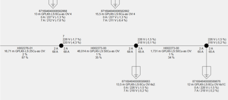
Future proof load model
The energy transition is causing major changes in the load on low-voltage connections (households, offices, shops, etc.). Until recently, the typical load on low-voltage grids was dominated by light bulbs, washing machines, refrigerators and televisions. Now more and more heat pumps, solar panels and electric transport are added, increasing the uncertainty of the load on a connection. In order to be able to adapt electricity grids to this energy transition, grid operators and distribution companies must be able to quickly calculate and analyze various scenarios. Strand-Axelsson's traditional load model is no longer suitable for this purpose.
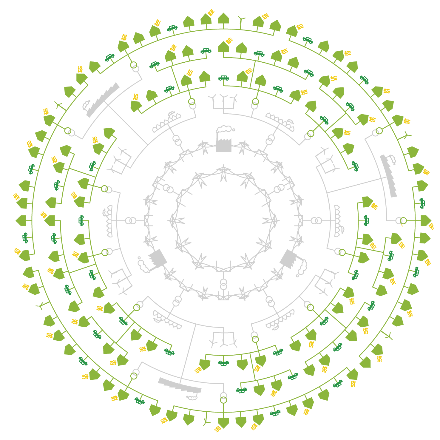
Phase to Phase has therefore developed an entirely new modular load model. With this model iy is possible to accurately calculate the future load on low-voltage networks. Moreover, it can be used to efficiently calculate various possible future scenarios. Using smart metering data, the model is easy to keep up to date.
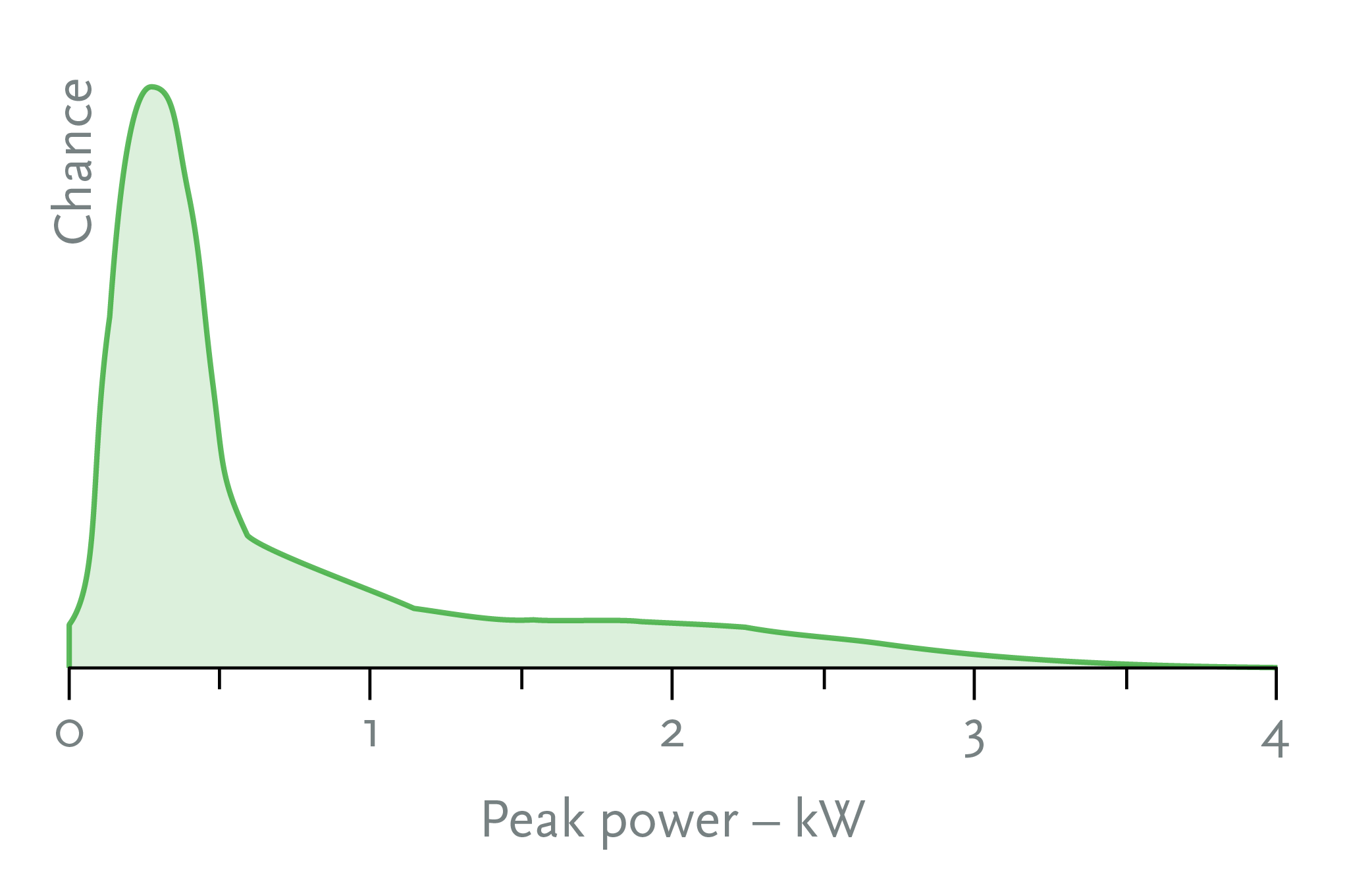
Standard load
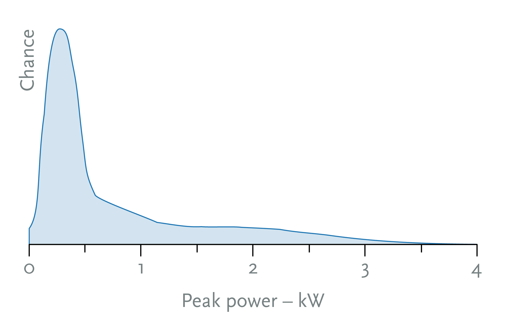
Smart metering data is used to determine the standard load per category (terraced and detached houses, apartments, commercial buildings, etc.).
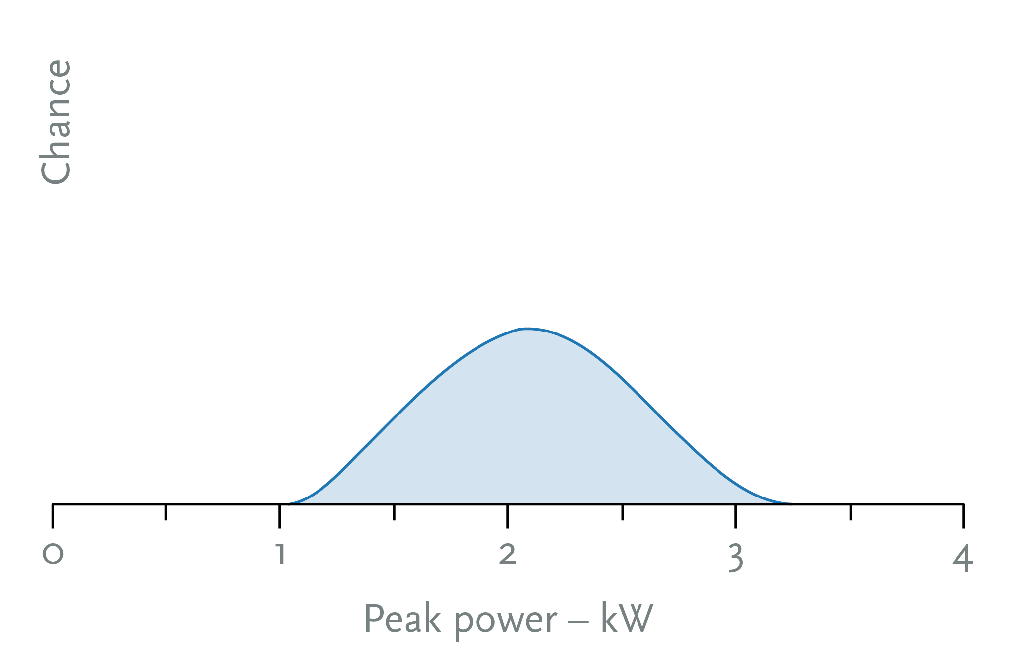
New additional loads
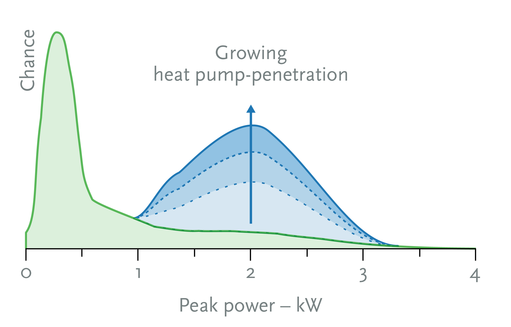
Heat pumps, solar panels, electric cars, etc. can all be modelled with one method and combined with the standard load.
Scenarios
With the combined load different scenarios can be created. Thus it quickly becomes clear in which grids problems are to be expected and where there is still sufficient space.
Self-learning
Smart metering data
More and more low-voltage grid measurement data is becoming available via the smart meter. These smart metering data show the current load of a connection. By allowing a model to learn from smart meter data, an accurate model of consumption is created. The model can be further trained for different types of connections, such as shops, detached houses and apartments by using specific smart meter data.
Training models
Load types can be trained using smart metering data or measurement data from individual devices. With more measurement data the models will become more accurate.
- Correlation between different devices can be included.
- The trend can first be filtered out of the data to separate the deterministic and stochastic part.
- An ε-accelerated expectation maximization algorithm is used for training.
Create load types
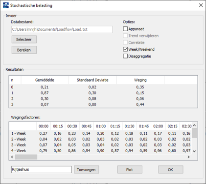
Different categories of smart metering data (e.g. apartments, detached houses) provide different models and device specific load models. This gives the user the freedom to create load types with the features most interesting to him.
Time
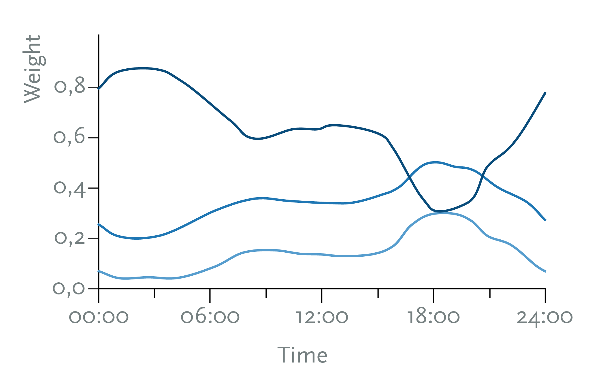
With smart metering data, the time variation in the load can also be taken into account. This makes it possible to determine the distribution of the load for each moment on a day. This is done with the weighting factors of the composite distributions that vary over the day.
Modular
Flexible modelling
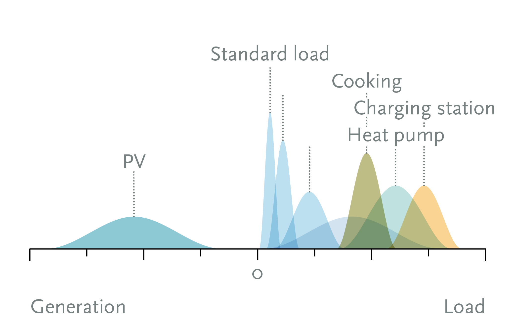
The loads in the new model are modelled as mixed normal distributions. By using mixed normal distributions instead of a single normal distribution, almost all distributions can be modelled. In this way, load types can be trained not only for households but also for shops, offices, etc.
Load types can also be adapted to local characteristics or from data from smart-grid pilots in order to simulate the effects of scaling up a pilot.
Combining different loads
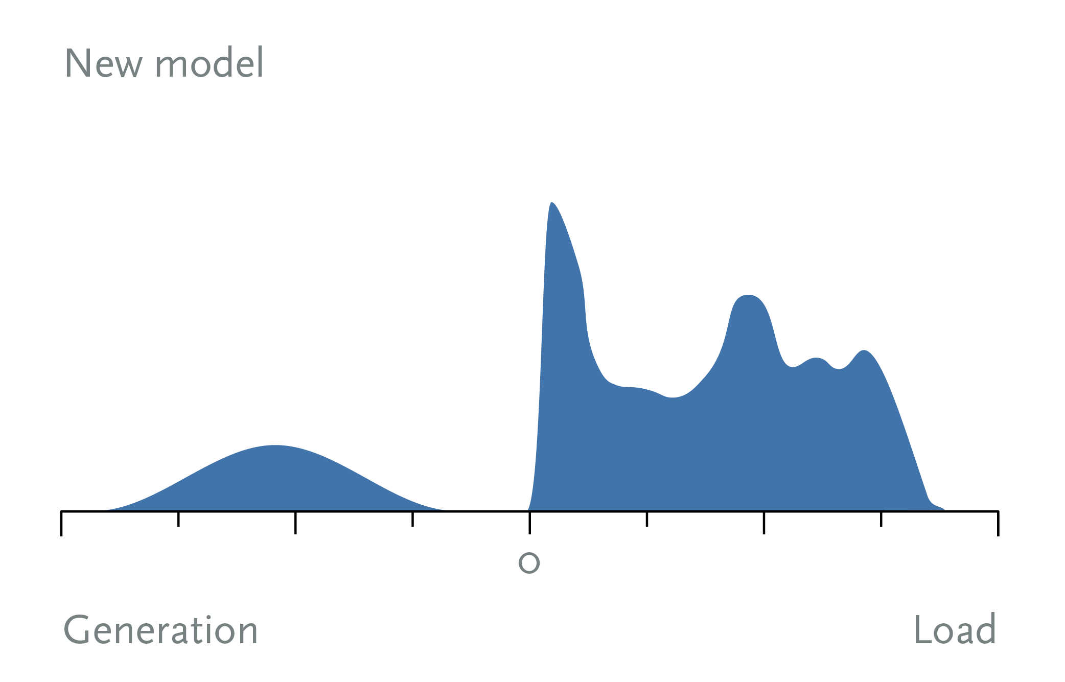
Different loads can easily be combined because each load is modelled in a similar way. This makes it easy to create and calculate different scenarios. This makes it possible to easily combine these loads into one new stochastic load.
Stochastic
Simultaneity
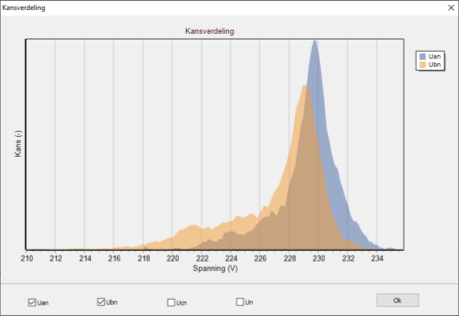
The stochastic load is determined at two moments: peak and valley (PV peak). Since the load is trained on household consumption data, the behaviour of the inhabitants can be taken into account. A probability distribution of the load is available for each household. For most calculations, the ideal calculation moment will first be determined.
- The load and PV peak can be determined grid-wide and per field.
- The load model incorporates time (day, year). This makes it possible to determine the load at any time with the correct simultaneity.
Load flow
- Stochastic load flow through Monte Carlo simulation.
- Linearization of the loads to accelerate the load flow.
- Equally fast as the current load flow for the stochastic load.
- Parallel calculations within the load flow.
- Orthogonal matrix-based Latin hypercube sampling.
- Quasi-stochastic load flow with deterministic results.
- Choice of percentile results or actual distributions.
Profiles
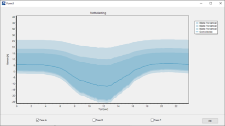
With sufficient smart metering data it is also possible to determine a profile with the load model. For the profile load flow, a large amount of smart metering data is needed, because one needs to make a prediction over a long period of time.
- In a profile calculation both stochastic and deterministic loads can be taken into account.
- The grid load is used to estimate the profile over the day.
Practice
Easy input
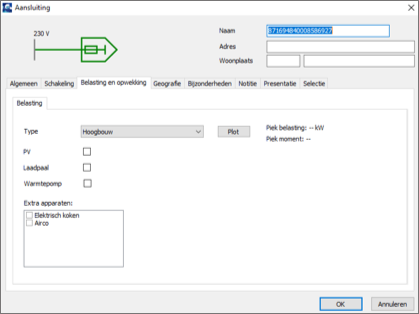
With the new load model, load input is very easy. All devices and the standard load are entered via the type file. It is therefore possible to add PV, EV charge points, heat pumps, etc. with a single click. In addition, the existing extended input is also available, so that – if available – detailed information can be entered.
Load types can be adapted to local characteristics or can be trained from data from smart-grid pilots in order to simulate the effects of scaling up a pilot.
Scenario calculations
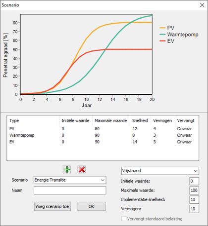
Scenarios can be defined, unrestricted, to determine whether the grid remains future-proof. Not only the penetration rates of specific appliances can be adjusted, but the standard household load can also be changed from one load type to another.
Scenario calculations can be used to display the probability of overload and voltage problems as a function of time.
Create scenarios
The results of the load flow and grid load calculations look exactly like you are already used to in Gaia. More elaborate stochastic results are also available for load flow and grid load calculations, which can be used for more detailed analyses.
- New loads (PV, heat pumps, etc.) no longer need to be modelled separately.
- Translation of local penetration rate to individual households.
- The chance that a household will have solar panels in the future, for example, is included in the stochastic load.
- A probability distribution can be built up for different penetration rates of specific techniques.
